
Introduction
Digital Twin technology is generally considered to be part of the wider Industry 4.0 revolution, whereby the digitalisation of various industries opens up new opportunities to exploit data to improve products and processes.
Digital twin
The term “Digital Twin” is widely used and has a range of accepted definitions. The term generally refers to an integration of data between physical and virtual components (Fuller et al., 2020). In the current context of the manufacturing process of gas turbine blades, a Digital Twin incorporates structured-light scans and aerodynamic performance (primary functional requirement) predictions. The scan data traces the unique geometry of each component and the aerodynamic predictions can be used to sentence components and compensate for manufacturing variability (Lee et al., 2019a).
Aerodynamic simulation hierarchy
The aerodynamic environment of a turbine blade is complex and can only be captured using physics-based simulations. Computational Fluid Dynamics (CFD) tools that encompass a range of fidelities have been used by various published studies and they will be discussed here in the order of increasing fidelity.
Considering the high volume of manufactured blades, rapid CFD tools like the Multiple blade Interacting Streamtube Euler Solver (MISES) (Drela, 1985) are attractive. MISES is a streamtube Euler solver coupled to an integral boundary layer code that is limited to quasi-three-dimensional (Q3D) blade sections. It has been used to assess compressor blades (Garzon and Darmofal, 2003; Dow and Wang, 2015; Goodhand et al., 2015) and turbine blades (Duffner, 2008).
Reynolds-Averaged Navier-Stokes (RANS) CFD solves the time-averaged Navier-Stokes equation. By incorporating source terms, turbulence models, and mixing planes, full three-dimensional (3D) geometries of multi-passage and multi-blade-row turbomachinery can be studied. However, RANS CFD is not able to resolve time-dependent phenomena and is vulnerable to turbulence and transition modelling. With today’s computational resources, RANS CFD is the favoured tool for predicting the aerodynamics performance of manufactured gas turbine blades (Lange et al., 2012; Högner et al., 2016).
Unsteady RANS (URANS) CFD allows time-accurate fluctuations in the flow field to be resolved. URANS can capture large-scale movements in the fluid but does not resolve the vortical structures in the boundary layer. In addition, the computational cost of URANS models often make them impractical for the purposes of design, let alone for high-volume assessments. If resources permit, URANS CFD could provide useful insights for dynamic blade loading (Clark et al., 2018).
The highest degrees of fidelity are offered by Large Eddy Simulations (LES) and Direct Numerical Simulation (DNS). These tools can resolve flow features at the length scales of surface roughness (Kapsis and He, 2018). However, given their immense computational cost, these are not currently practical options for Digital Twins, and are therefore not considered in this paper.
Increasing the fidelity of the CFD methods improves the realism and accuracy of the predictions but it is also associated with higher computational cost and complexity. Given the high volume of parts that need to be assessed, a balance must be struck between computational expense and accuracy. This paper therefore examines the question: what is the trade-off between cost and accuracy of different aerodynamic simulation fidelities?
Paper aims & outline
This paper compares the accuracy and computational cost of a range of aerodynamic simulation methods. Using the geometric data from a set manufactured turbine blades, the predictions of key aerodynamic performance parameters are compared across the range of simulation fidelity. The following sections detail:
the aerodynamic simulation methods;
the geometry measurement and processing methods, and;
the results obtained from the various simulations, highlighting differences in capability and cost.
The paper concludes with recommendations on the suitable aerodynamic simulations to support Digital Twins.
Methodology I – aerodynamic simulation methods
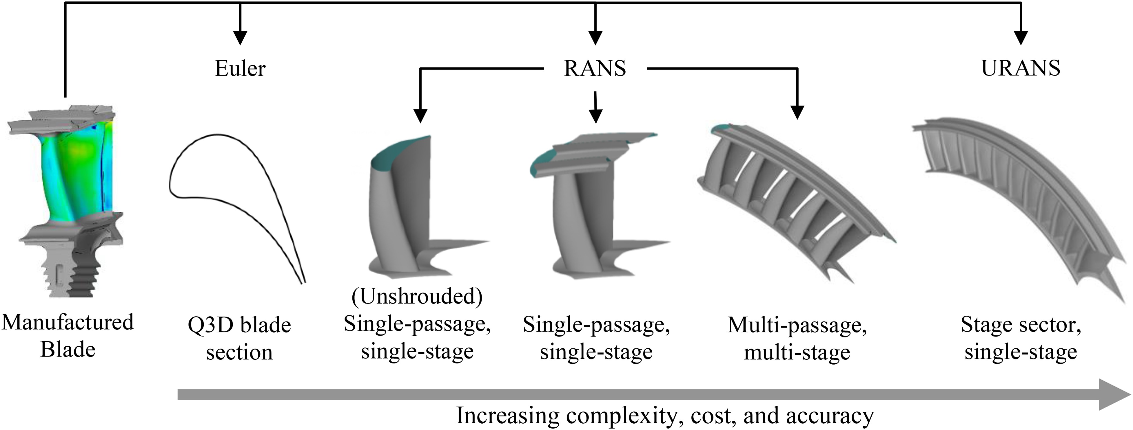
The aerodynamic simulation methods that are considered in this paper are shown in Figure 1: Euler models, unshrouded and shrouded single-passage-single-stage RANS models, multi-passage-single-stage RANS models, single-passage-multi-stage RANS models, and single-stage URANS models. MISES was used as the Euler solver and Rolls-Royce’s in-house CFD solver, Hydra (Moinier and Giles, 1998), was used for the RANS and URANS models.
The approach taken for this study is purely computational. It would also be possible to experimentally test parts with manufacturing variability and compare the results to the predictions from simulations. However, many of the performance changes observed are within the accuracy range of even very well-conditioned experiments, especially when compressibility effects are considered. The paper therefore ultimately references the simulations to the highest fidelity case (the URANS models).
Euler solver: MISES
Version 2.56 of MISES was used and the models were run to the prescribed pressure ratio. The models were run for 10 inviscid iterations before introducing viscous effects for a further 15 iterations. This made the model more robust by allowing the flow field to stabilise before introducing the boundary layers (Drela and Youngren, 2008).
RANS solver: Hydra
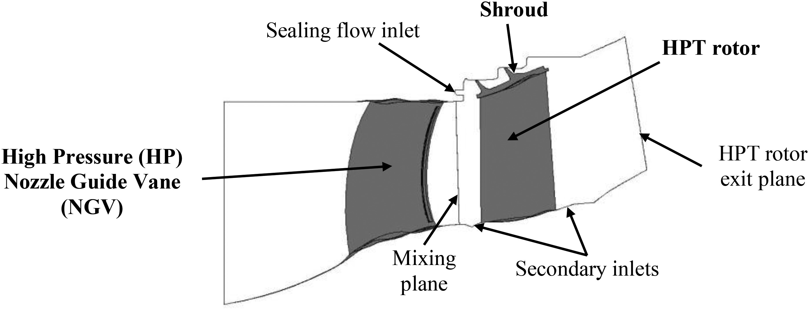
Hydra’s spatial discretisation is based on an upwind edge-based finite volume scheme and is second-order accurate. Hydra has been experimentally validated for a similar geometry (Zamboni and Adami, 2016) and across a range of turbine designs (Coull, 2017). Rolls-Royce’s Parametric Design & Rapid Meshing (PADRAM) (Shahpar and Lapworth, 2003) was used to generate multi-block, structured meshes. Unless otherwise specified, the computational domain is a 1-stage simulation of the High Pressure Turbine (HPT) stage, as illustrated in Figure 2. Sealing flows and film cooling are modelled using secondary inlets and source terms on the blade respectively.
The
Figure 10.
Plots of the averaged single-passage (ASP) values against multi-passage (MP) values from the multi-passage CFD models for the: (a) mass-averaged β exit ψ η

This approach contains approximations, including: the inability of RANS models to resolve time-dependent phenomena (e.g. TE shedding), film cooling being represented by source terms, and the turbulence model. Broadly speaking, these uncertainties behave systemically and assuming a uniformly distributed impact on the results, the effect of these approximations on the predicted performance changes from the design-intent is significantly reduced.
Key performance parameters
For a turbine stage, the performance quantities of interest are: the exit flow angle,
For the purposes of this study,
(3)
Methods II – geometry measurement and recreation methods
The ability to capture and recreate the geometry of manufactured blades in a numerical environment is essential for the Digital Twin. Suitable measurement methods include using a Coordinate Measuring Machine (CMM) (Garzon and Darmofal, 2003), structured-light scanning (Heinze et al., 2014), and computed tomography (Högner et al., 2017). Structured-light scanning is the method of choice as it produces tessellated point clouds, stereolithography (STL) meshes, with an accuracy of
The geometric information from the STL meshes need to be extracted before it can be mapped to the relevant input files for MISES and PADRAM and this is shown in Figures 3 and 4. The STL meshes were first aligned using the fir tree (highlighted red in Figure 3) in order for the blades to be oriented as they would be in the engine. Since film cooling is modelled with source terms, a smooth blade surface is required and the film cooling holes were removed using BladeCleaner (Högner et al., 2015). Blade sections were then extracted at 21 circumferential stream surfaces. The as-scanned trailing edge (TE) steps cannot be modelled in MISES and they tend to introduce negative volumes in the PADRAM mesh. Thus, a circle was fitted in the vicinity of the TE and the TE step was omitted. The result is blade sections that preserve the geometry of the STL meshes, except in the region of the TE. This simplification is a source of uncertainty due to the limitation of using a structured meshing approach that is more suitable for parametrically defined blades.
Figure 3.
The geometry recreation process including: STL mesh alignment, film cooling holes removal, blade sections extraction, and removal of the trailing edge step.
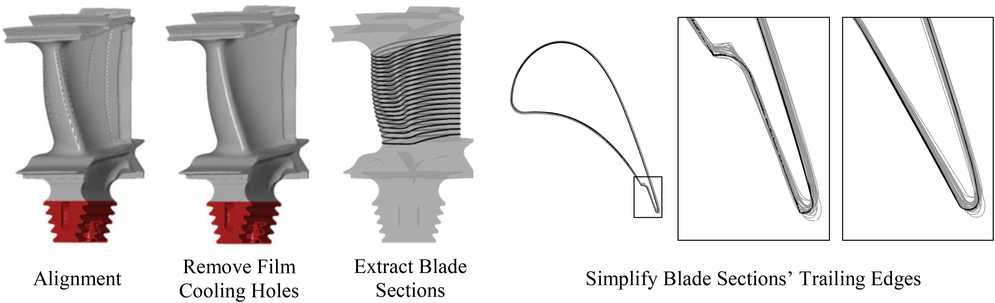
Figure 4.
(Left) Mapping the measured blade geometry to the MISES and PADRAM blade sections. (Right) Displacement fields from an example STL mesh and its reconstruction in PADRAM.
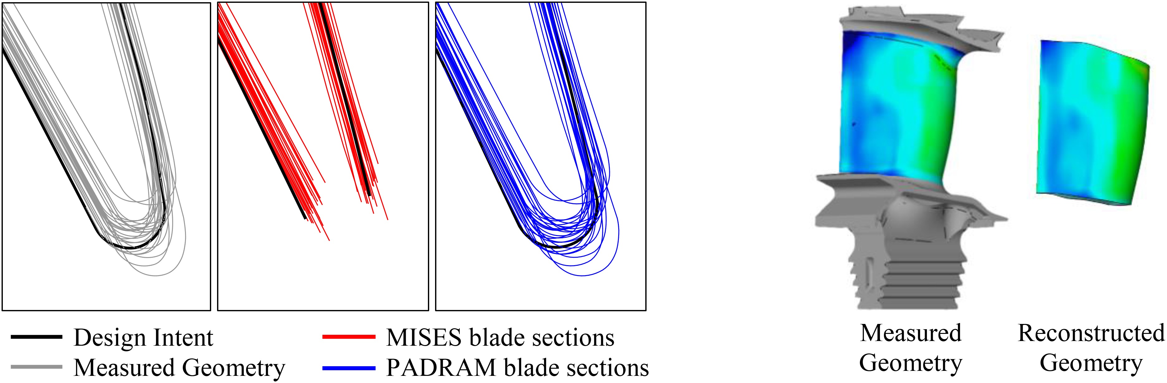
Displacement fields were obtained by comparing the blade sections from the STL meshes to the design-intent. As the blades are manufactured “cold” and the engine runs “hot”, the displacement fields were scaled to account for thermal expansion by comparing the corresponding chord lengths between the physical and CFD blades. The scaled displacement fields were then mapped to the MISES and PADRAM blade sections, as shown in Figure 4 (Left). The span-wise geometry change is also well captured and this can be visualised by comparing the displacement fields from the STL mesh and the PADRAM reconstruction, as shown in Figure 4 (Right). Since MISES does not model the TE, the MISES blade sections were “cut-back” by
Results and discussion
The results obtained from the various aerodynamic simulation methods will be discussed under the following topics, which compare the methods in Figure 1 in the order of increasing fidelity:
Part I: Q3D Euler vs. Single-Passage 3D RANS
Part II: Multi-Row and Multi-Stage Effects
Part III: Multi-Passage Effects
Part IV: Accuracy and Computational Costs across the Hierarchy
Part I: Q3D Euler vs. single-passage 3D RANS
The ability to accurately predict the
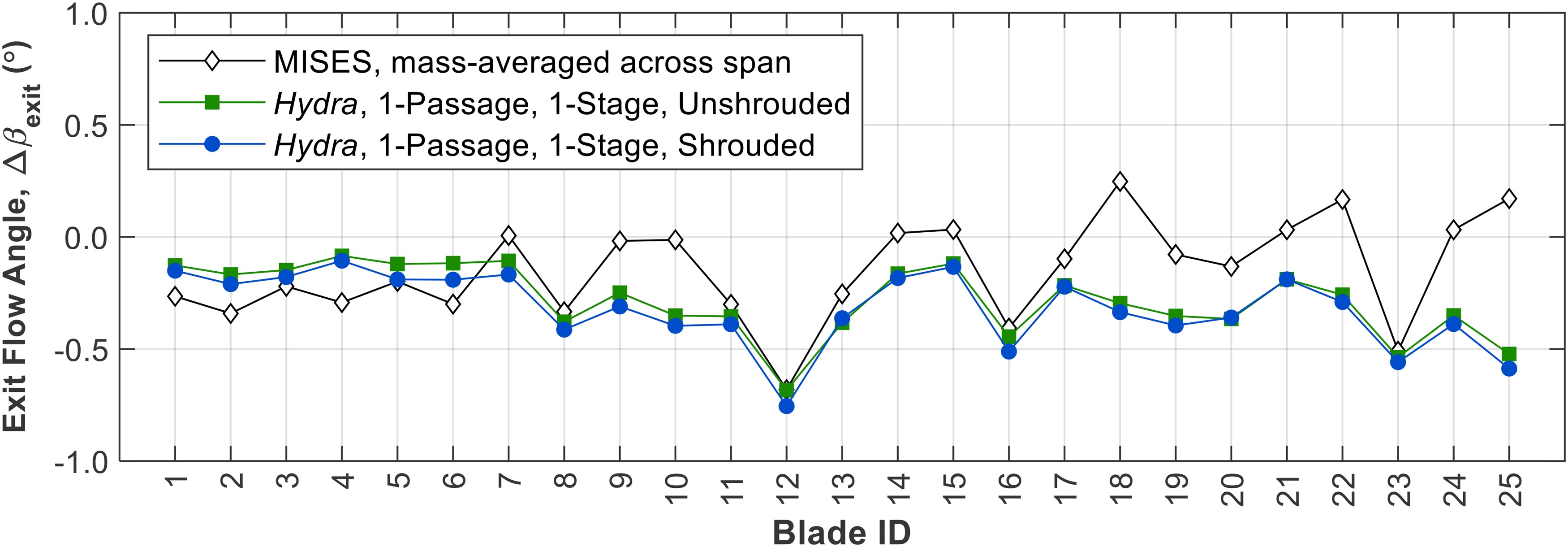
Q3D MISES models from the 21 blade sections extracted from each blade.
3D, unshrouded, 1-passage, 1-stage, Hydra RANS model.
3D, shrouded, 1-passage, 1-stage, Hydra RANS model.
The MISES results were mass-averaged across the span and the Hydra results were mass-averaged at the HPT rotor exit plane. Figure 5 shows that the trend from MISES does not match those of the 3D Hydra models completely and with notable discrepancies for blade IDs 18, 24, and 25. This is primarily due to MISES treating each Q3D blade section in isolation and not accounting for the effects of the hub and tip vortices. In addition, the trends from the unshrouded and shrouded models show that changes in the
Part II: multi-row and multi-stage effects
For civil aero engines, the aerodynamic changes on one blade row will have a “knock-on” effect on all downstream blade rows. To study this, 3D RANS CFD models of an extended computational domain were created, incorporating the Intermediate Pressure (IP) NGV, Intermediate Pressure Turbine (IPT) rotor blade, and the first Low Pressure (LP) NGV. Figure 6 shows the radial profiles of the inlet and exit flow angles, referenced to the mass-averaged values across the respective inlet and exit planes, and gives a visual appreciation of the how small geometry changes in the HPT rotor blade row affects the flow angles of the entire IPT stage (IP NGV and IPT rotor blade).
Figure 6.
Radial profiles of flow angles from the HPT rotor exit and the IPT stage. “Abs.” denotes “absolute” and “Rel.” denotes “relative”. Refer to Figure 8 for the corresponding efficiency plots.
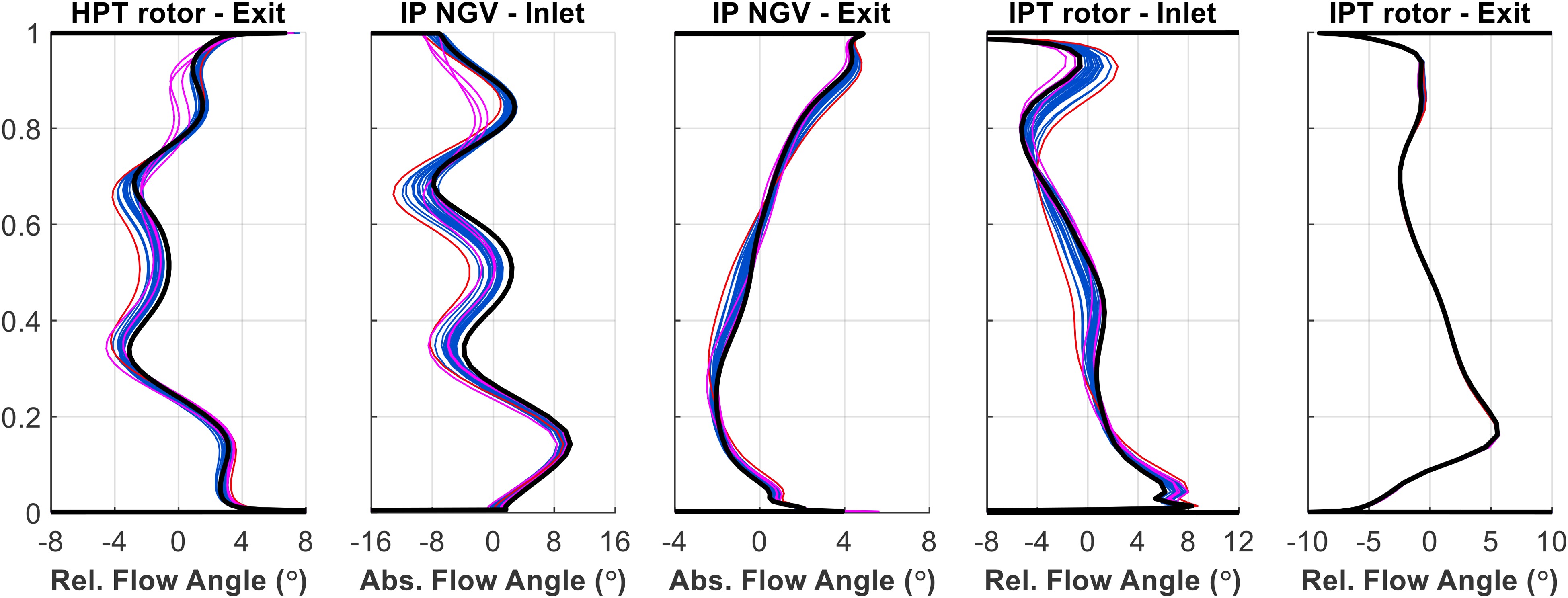
Although the geometry changes were only imposed on the HPT rotor blade, Figure 6 shows that the downstream effects only diminish by the IPT rotor blade exit. Immediately downstream of the HPT rotor, the flow angle changes caused by the geometric variability imposed on the HPT rotor blade lowers the inlet flow angle to the IP NGV (in the absolute frame) by up to
Examining the radial profile of
Figure 7.
Illustration of the flow structures due to the blades’ proximity to the cavity, showing (Left) the HSV partly in the cavity and (Right) the HSV outside the cavity.
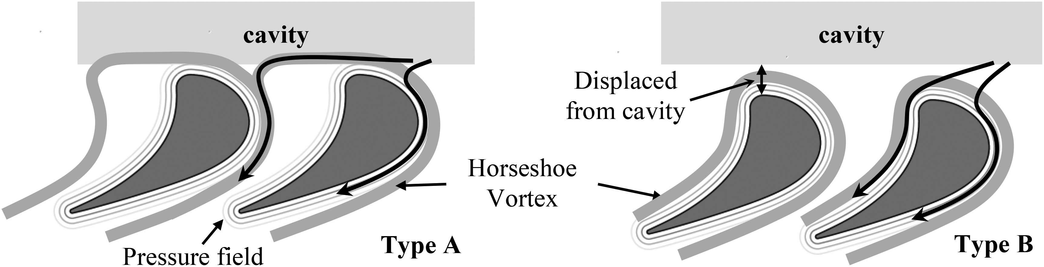
If the influence of the blades’ pressure field is weakened, either by a change in blade loading and/or a change in the position of the blade, the pressure side leg of the HSV emerges from the cavity and wraps around the blade leading edge. This alternative mode for the HSV is shown in Figure 7 as “Type B” flow. A more detailed discussion surrounding the mechanism behind this change in the flow field has been previously published (Lee et al., 2019b).
The changes in the flow angles in the IPT stage affects the efficiency of the stage and Figure 8 plots the changes in the scaled
Figure 8.
Scaled stage efficiencies obtained from the 1-stage and 2.5-stage Hydra RANS models. Refer to Figure 6 for the corresponding radial profiles of the flow angles.
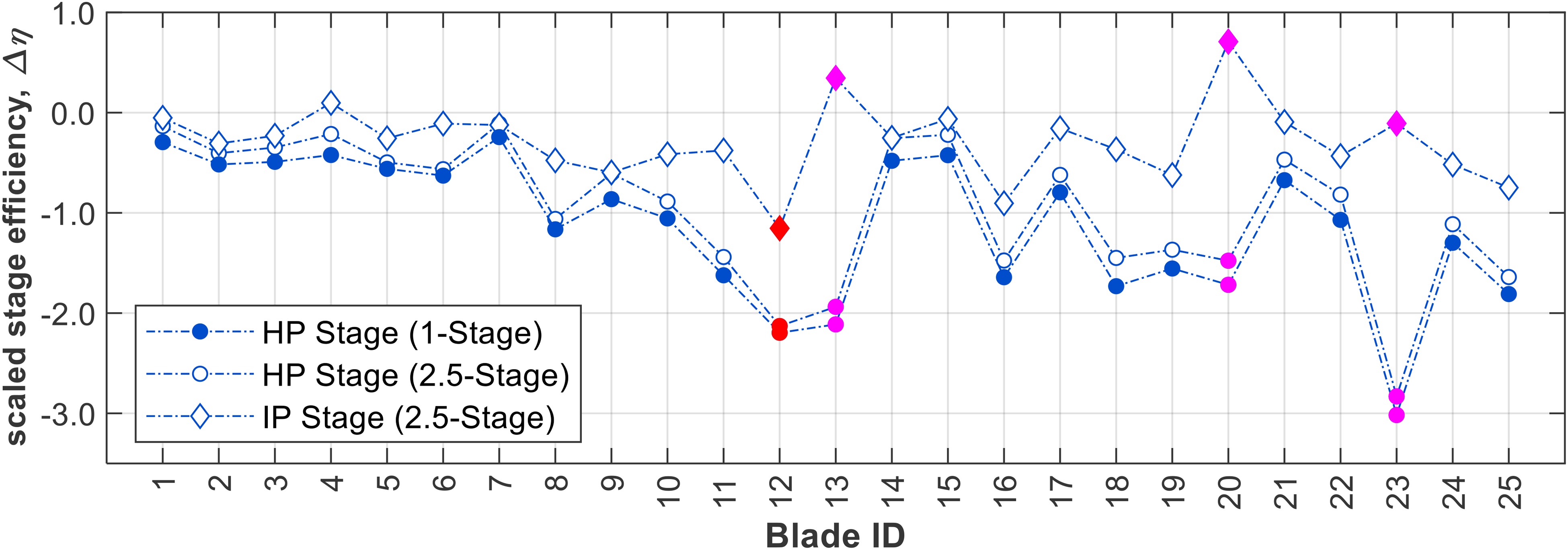
Red: Blade ID 12 exhibits Type A behaviour and both the HP and IP stage scaled
Magenta: Blade IDs 13, 20, and 23 exhibit Type B behaviour but only the HP stage scaled
For blade ID 12, the HPT rotor exit flow angle was significantly reduced between
For blade IDs 13, 20 and 23, the change in HSV behaviour causes the tip region of the HPT rotor blade to under-turn the flow, producing less work and reducing HPT stage efficiency. However, unlike for blade ID 12, the IP NGV is effective is removing most of the flow angle discrepancy at the IP NGV inlet and the exit flow angle from the IP NGV is similar to the design-intent, minimising the impact of the change in HSV behaviour on the IPT stage efficiency.
The small differences in the trends between the 2.5-stage and 1-stage predictions of scaled
Part III: multi-passage effects
In an engine, adjacent blades will have slightly different manufacturing deviations. This interaction with neighbouring blades is not captured by single-passage calculations which assume periodicity over one blade pitch. Multi-passage simulations were therefore used to explore these interactions: 26 1-stage models each of 3-passage and 5-passage shrouded HPT rotor blades were created and solved using Hydra. The 26 cases include one case (case index 1) assembled using only blades that exhibit Type B behaviour, and a further 25 cases constructed using Latin Hypercube Sampling where geometric data from the 25 STL meshes were used to populate each blade position once.
As with the single-passage calculations, multi-passage cases also exhibited Type A and Type B flow. However, the flow structure for each multi-passage calculation does not simply depend on the presence of blade(s) that exhibited Type B behaviour in a single-passage calculation. Figure 9 compares:
Figure 9.
Flow structures observed in the multi-passage (MP) CFD models and the “average” flow structure from the single-passage (ASP) CFD models of the corresponding constituent blades.

the flow structure observed in the multi-passage calculations (subscript MP) and
the “average” of the flow structures that are observed in the single-passage calculations (subscript ASP) of the corresponding constituent blades.
Examining the trend for the 5-passage cases, Type B flow is observed in multi-passage cases 1, 3, 5, 6, 7, 9, 12, 15, 17, 18, 23, and 24 but cases 6, 9, 12, and 24 do not contain blade(s) that gave Type B behaviour in a single-passage calculation. In addition, multi-passage cases 10, 14, 16, 21, 25, and 26 all contain a blade that gives Type B behaviour but all demonstrate Type A flow. Similar observations can be made for the 3-passage cases.
The above comparison shows that the detailed flow behaviour in the multi-passage environment is somewhat different to the single-passage environment. Nonetheless, if the overall performance can be estimated from an average of single-passage calculations, then the cost and complexity of simulations will be reduced enormously. Figure 10 shows this assessment for the four key performance parameters mentioned earlier:
each subplot compares the multi-passage (MP) result with the average of single-passage (ASP) results;
the accuracy of the averaging is quantified using an
the mean and standard deviation of the MP and ASP predictions are indicated by a circle marker and error bar respectively along the appropriate axes.
Figure 10a and 10b show good agreement between the ASP and MP results for the mass-averaged
In contrast, Figure 10c shows significant discrepancy between the predicted stage loading
To summarise, the HSV flow structure near the vicinity of the HPT rotor blade tip is bimodal: Type A and Type B flow are observed as two distinct states with no clear intermediate state between the two. The behaviour is sensitive to interaction between adjacent blades and their pressure fields. Considering overall performance parameters, flow angle and capacity are well approximated by averaging the individual single-passage predictions of each blade
Part IV: accuracy and computational costs across the hierarchy
Having examined some of the differences between the predictions obtained from aerodynamic simulation methods of various degrees of realism, attention now returns to the central question motivating this paper, namely what is the trade-off between cost and accuracy of different aerodynamic simulation fidelities?
Figure 11 plots the predicted changes in capacity
Figure 11.
Comparison of the computational costs (CPU core hours) and the predicted performance changes by the various aerodynamic simulations across the aerodynamic simulation hierarchy.
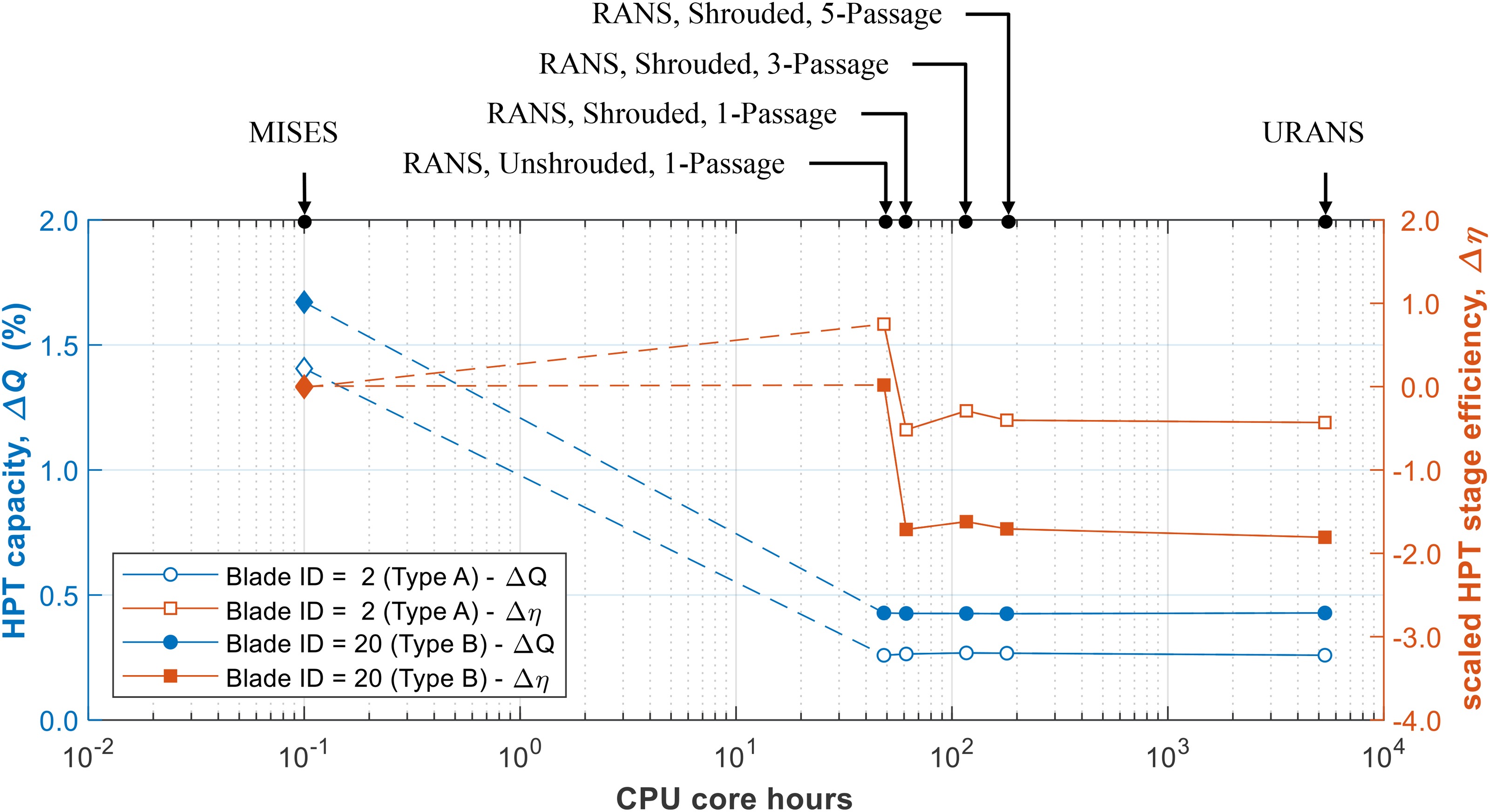
On a log-scale, the Euler, RANS, and URANS CFD models occupy three distinct regions. Compared to the predictions from RANS and URANS, Euler models are very quick and take only ∼15 CPU core seconds per blade section. However, the Euler models fall short in the ability to capture the performance changes observed in the higher fidelity methods. The RANS models are all of similar order of magnitude in terms of simulation cost (50–200 CPU core hours) and the URANS models require ∼5,500 core hours. As the URANS models required the same size sector for the NGV and rotor blade rows, the URANS models had 6 HP NGVs and 11 HPT rotor blades. In addition to these raw computational costs, the complexity in running the models in Figure 11 generally increases with fidelity. Rising computational cost is therefore accompanied by an increase in the time and expertise required to build and manipulate these models.
As a general principle, the required aerodynamic modelling fidelity is driven by the need to capture the aerodynamic phenomena that drive the performance quantities of interest. While it is difficult to draw more specific universal rules for simulation, the following recommendations can be made for Digital Twins of gas turbine blades (in particular, a HPT rotor blade):
For predictions of capacity Q and mass-averaged flow angle
For the predictions of stage loading
The approach of using URANS CFD models to support a Digital Twins seems unnecessarily complicated and costly as the predicted performance changes no longer vary significantly beyond a single-passage, shrouded RANS CFD model.
As a general design rule, components should have a robustness to variability. The blade tip could be designed to stabilise the HSV structure which would improve the reliability of lower-fidelity models and reduce the required complexity in the aerodynamic simulations.
Conclusions
Using MISES and Hydra, CFD models of varying degrees of realism were generated and the performance of 25 scrapped HPT rotor blades was assessed. The goal was to determine the required level of fidelity in simulations to obtain physics-based predictions that can be used to support Digital Twin technology for the manufacturing process of gas turbine blades. The performance of the HPT stage was quantified in terms of the rotor exit angle
In terms of the bulk flow properties, MISES, although quick, was unable to capture the trend in
Multi-passage calculations were performed to assess interactions between neighbouring blades and these interactions affect the casing horseshoe vortex behaviour. In general, flow angle
To support Digital Twins of a HPT rotor blades, an unshrouded single-passage 3D RANS model is sufficient to assess flow angle and stage capacity changes, while a shrouded single-passage 3D RANS model is the minimum required fidelity to give an estimate of stage loading and efficiency. The fidelity of the CFD models could be reduced if the casing flow structure change were avoided by designing a blade that stabilises the horseshoe vortex. URANS simulations are far too costly for extensive use, but serve as a useful benchmark for this study.
Nomenclature
Difference
Exit flow angle
Stage efficiency
Viscous shear
Stage loading coefficient
Tangential component of force
Stagnation pressure at stage inlet
Stage inlet capacity
Surface
Stagnation temperature at stage inlet
Blade velocity
Tangential velocity
Axial velocity
Total enthalpy
Mass flow
Mass flow at stage inlet
Static pressure
Radius
Abbreviations
3D
Three-Dimensional
ASP
Average of Single Passage
CFD
Computational Fluid Dynamics
CMM
Coordinate Measuring Machine
CPU
Central Processing Unit
DNS
Direct Numerical Simulation
HP
High Pressure
HPT
High Pressure Turbine
HSV
Horseshoe Vortex
IP
Intermediate Pressure
IPT
Intermediate Pressure Turbine
LES
Large Eddy Simulation
MISES
Multiple blade Interacting Streamtube Euler Solver
MP
Multi-Passage
NGV
Nozzle Guide Vane
PADRAM
Parametric Design & Rapid Meshing
Q3D
Quasi-Three-Dimensional
RANS
Reynolds-Averaged Navier-Stokes
STL
Stereolithography
TE
Trailing Edge
URANS
Unsteady Reynolds-Averaged Navier-Stokes