
Introduction
Modern civil and military aircraft concepts often feature short and highly contoured engine intake systems. The reduction of overall aircraft drag lies in the focus of the civil boundary layer ingesting (BLI) aircraft concept, while the hiding of the highly reflective fan plane from a direct line of sight motivates military applications. As the flow passes through these ducts, secondary flows arise due to surface curvature and changes in cross-sectional area and shape. Towards the Aerodynamic Interface Plane (AIP) between intake and compressor, total pressure and swirl distortion arise. The subsequent compressor working under these inhomogeneous inflow conditions experiences losses in efficiency and performance. A reduced stall margin leads to the risk of engine surge and severe damage of the engine.
In the usual design process, the intake geometry is designed in an isolated approach using numerical simulations and wind tunnel experiments. The assessed AIP flow distortion is then quantified by distortion parameters, which are compared to safety limits specified for the subsequent engine.
A compressor working under non-uniform inlet conditions shows complex flow physics (Longley and Greitzer, 1992). Three types of inflow distortions exist: total temperature, total pressure, and swirl distortion. In the case of bent intake ducts, only the latter two are of relevance. An incoming swirl distortion changes the incidence angle of the compressor blades which directly impacts the local blade work input in terms of total pressure and total temperature rise. Severe incidence angles may provoke stall and engine surge. An incoming total pressure distortion is always related to a distortion in axial velocity in the distorted sector. It changes the
In recent years, full annulus URANS simulations of (multi-stage) compressors working under distorted inflow allow a detailed investigation of the highly three-dimensional character of the flow field (Yao et al., 2010a,b). First, simple generic distortion patterns were investigated and compared to experimental data (Gunn et al., 2013; Lesser and Niehuis, 2014). Later also BLI typical distortion patterns have been investigated which feature both radial and circumferential total pressure profiles (Gunn and Hall, 2014). Weston et al. (2015) investigated the transport of the inflow distortion through a three stage fan, while recently, Page et al. (2017) focused on complex combined pressure swirl distortions like they also occur in bent intake ducts.
Within the scope of a research project, an experimental full size intake-engine test case was set up at the Bundeswehr University Munich. Experimental data was collected allowing detailed insight into the intake flow field and the AIP flow conditions. In the present publication, the abilities of three different numerical approaches in reproducing the measured flow field are evaluated: An isolated intake simulation, isolated full annulus low pressure compressor (LPC) simulations exposed to the measured AIP flow field, and finally a coupled approach of intake and LPC.
Experimental test case
In cooperation with MTU Aero Engines AG, the Institute of Jet Propulsion set up an experimental test case combining a generic highly contoured intake geometry and a state of the art MexJET turbofan engine (Rademakers et al., 2016). A schematic sketch of the intake and the three stage low pressure compressor section of the setup is given in Figure 1.
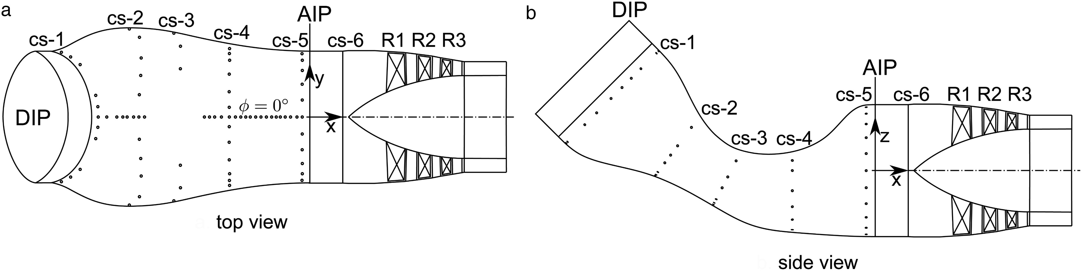
Prior to entering the intake at the duct inlet plane (DIP), the flow is guided through an airmeter, which is not shown in the drawing for reasons of clarity. A traversable measurement rake equipped with five-hole and pitot probes is part of the measurement equipment. It can be installed at the DIP to measure the inflow, needed as inlet boundary condition for CFD, or at the AIP to measure the duct flow distortion. In both cases, static and total pressures as well as the flow angles are measured at 120 positions within the respective plane. Due to the limited calibration range of the five-hole probes, flow angles larger than ±30° cannot be measured. Close to the wall, the total pressure is captured by three pitot probes at 24 circumferential positions. The inflow conditions are additionally measured by two boundary layer probes at
The intake flow field lies in the focus of the present numerical investigations. The measurement equipment within the LPC only consists of total temperature as well as static and total pressure probes at four circumferential positions at the LPC outlet. This allows the assessment of the operation point
CFD setup
The flow solver TRACE (Nürnberger, 2004; Kügeler, 2005) is used for the presented CFD simulations. This 3D finite volume code is developed at DLR-AT and was recently validated for full annulus calculations of low pressure compressors working under distorted inflow conditions (Lesser and Niehuis, 2014; Schoenweitz and Schnell, 2016). It solves the discretized (U)RANS equations on structured multi-block meshes. Fully turbulent mode was used due to Reynolds numbers of 5.25 · 106 and 2.52 · 106 based on intake diameter and fan blade chord respectively.
Due to the lack of a best practice setup for bent intake ducts an extensive numerical parameter study including a mesh density study was carried out (Kächele et al., 2018). It showed the superiority of the streamline curvature correction proposed by Kožulović (Kožulović and Röber, 2006) for the k-ω turbulence model within the duct domain.
Within the compressor domain, turbulence is modelled by the Wilcox k-ω model with an additional correction for rotational effects proposed by Bardina and a stagnation point anomaly fix according to Kato-Launder (Kožulović et al., 2004). Applied on a full annulus simulation of all three LPC stages, the standard mesh density, which is used for the calculation of speed lines and calibrated by rig experiments, would exceed the limited resources available in industrial applications. Thus, a coarsening of the temporal and spatial resolution of the simulation was necessary. These efforts towards a setup, which is still able to reproduce the dominant flow features of the intake-compressor interaction, are summarized by Kächele et al. (2016). A smart coarsening of the blade rows downstream of Rotor 1 leads to a reduction of overall cell count by 70% to 100 million cells with a similar reproduction of the speed line in the operational point of interest. A relatively coarse time step of 36 outer time steps per fan blade passage was still able to reproduce the desired rotor-stator interactions. In coupled performance runs the calculation time for one rotor revolution on the available 128 CPU was reduced to less than 2 days. This is necessary to account for the long expected transient oscillation time of the low frequent duct flow field of 12 to 15 rotor revolutions.
Isolated intake simulation
Isolated pre-test investigations (Kächele et al., 2018) indicated a weak unsteady behavior of the intake flow field. Its temporal average is thereby similar to the result of a steady simulation. Hence, no URANS computations are required for the assessment of the main isolated intake flow features such as the vortex system and the AIP flow field.
Inflow boundary condition
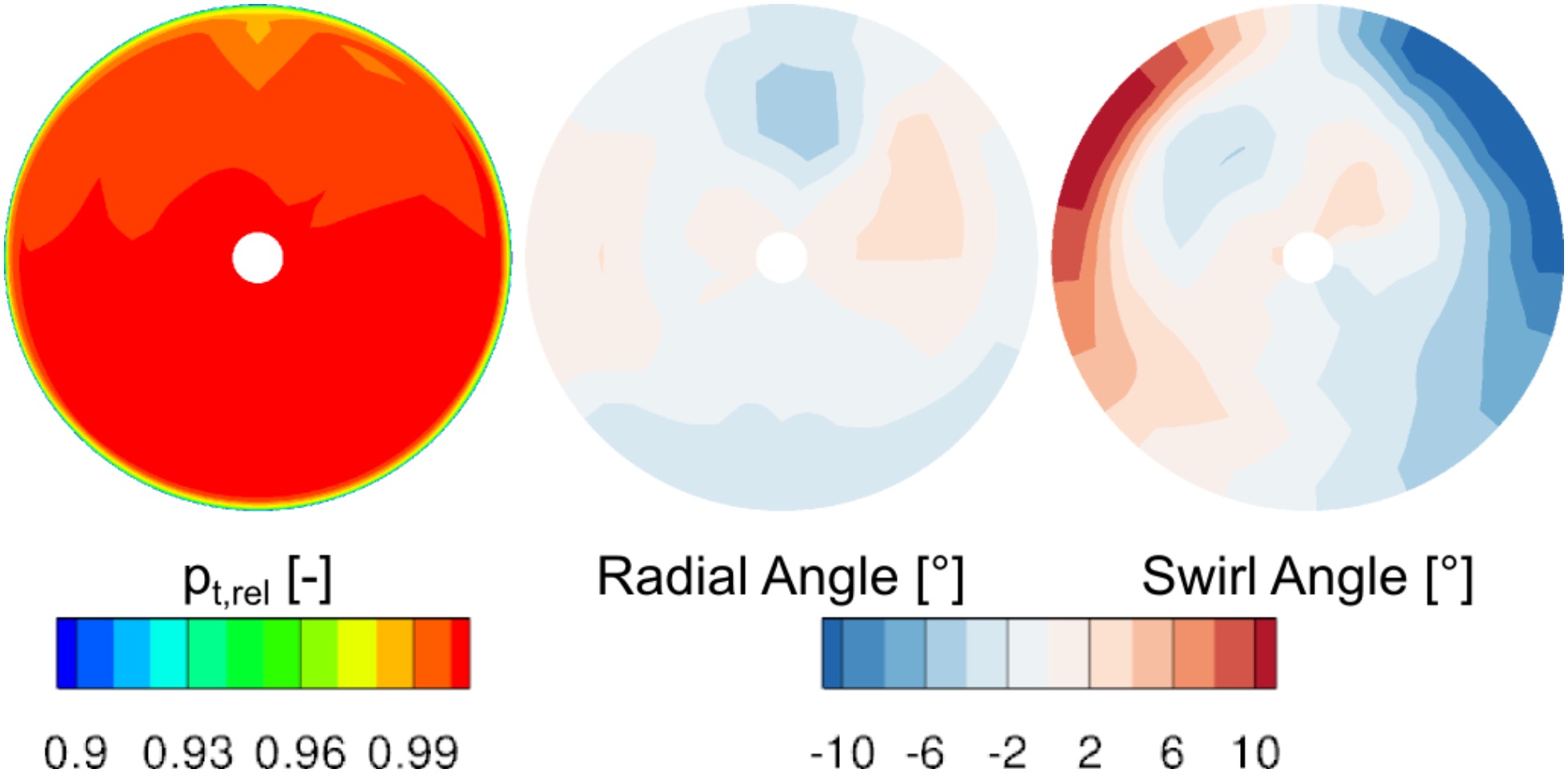
The measured DIP flow field shown in Figure 2 is used as inlet boundary condition. The local region of low total pressure close to the top of the DIP is the wake of a total temperature probe mounted shorty upstream. A swirl pattern with flow angles up to 15° arises due to the unconventional aerodynamics of the engine test facility (Muth et al., 2009). Flow angles measured by the five-hole probes at the outermost radial position are kept constant towards the outer DIP wall. Constant values for total temperature and turbulence level of 1.3% are taken from measurements. The necessary turbulent length scale is set to achieve a nearly constant turbulence level within the contracting part of the intake.
Comparison of CFD and experiment
The desired mass flow rate is set by adjusting the constant static pressure (“Duct OD outlet” in Figure 3) at the outlet boundary condition
Figure 3.
Comparison of experimental and CFD static wall pressure data along the centerline for the isolated and coupled intake simulation.
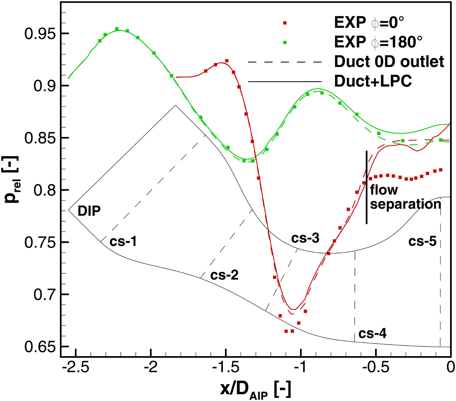
The intake flow field is determined by streamwise and cross flow pressure gradients that arise through centerline curvature and changes of cross-sectional area. In order to illustrate the relation between geometry and pressure gradients, the duct contour is added in the plot of the static wall pressures along the symmetry line in Figure 3.
Within the first half of the duct until cs-3 the cross-sectional area is reduced to 75% of the inlet area
Both geometric trends reverse in the second half of the duct: cross-sectional area increases, while the duct surface on the upper side experiences a strong curvature in positive z-direction. These two changes in geometry lead to a significant adverse streamwise pressure gradient at
Figure 4.
Comparison of experimental and CFD static wall pressures at cross-sectional planes cs-4 and cs-5.

The AIP total pressure distortion given in Figure 5 is mainly a result of the accumulation of low momentum boundary layer material due to secondary flow and additional losses caused by the flow separation. In the measured data, this distortion is accompanied by a static pressure distortion at the same position. This compressor induced static pressure field leads to a mass flow redistribution visible as radial and circumferential flow angles towards the center of the static pressure distortion. The constant static pressure outlet condition
Figure 5.
Comparison of experimental AIP flow field with results from the isolated intake simulation with constant outlet pressure (0D outlet), two dimensional outlet pressure (2D outlet) and the coupled simulation (Coupled setup).
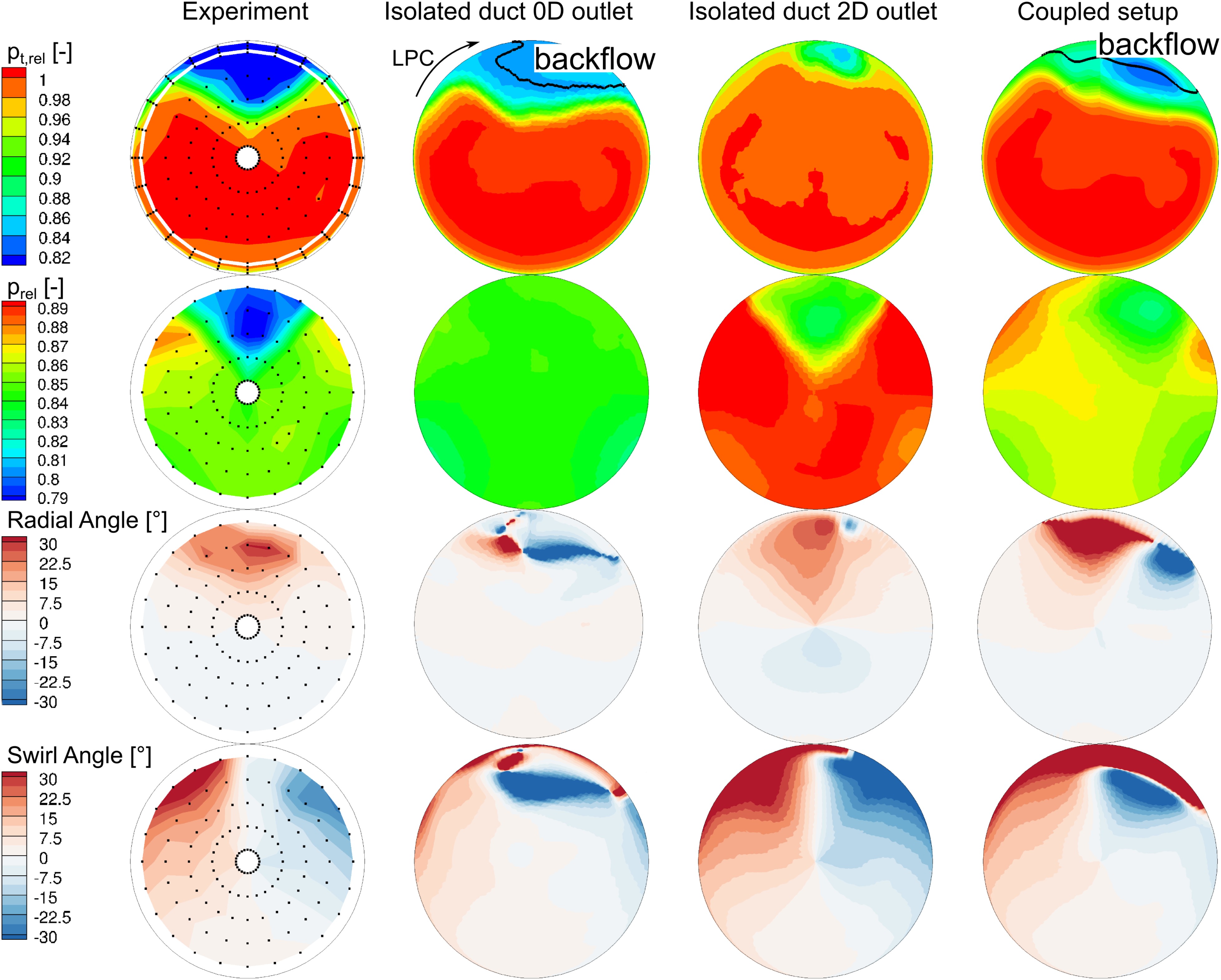
Even though the total pressure field is only slightly asymmetric, the region of backflow and hence the swirl distortion shows a significant asymmetry. In case of a homogeneous axial inlet boundary condition with constant flow variables, the AIP distortion pattern is 100% symmetric (cf. (Kächele et al., 2018)). It can thus be concluded that the intake flow simulation is very sensitive to asymmetries.
The measured AIP static pressure field can also be used as a boundary condition for the isolated duct domain (“Duct 2D outlet”). For such computations, the outlet boundary condition has to be placed within the AIP which reduces the possible extension of the flow separation. Again, the mass flow was set by adjusting the static pressure in cs-1. Using the original measured pressure field leads to an over prediction of the mass flow. Hence, the outlet profile was scaled to a higher pressure level by 5.2%. The resulting AIP flow field (cf. Figure 5) shows significant improvements concerning the flow angle distribution. The total pressure distribution, however, is reduced both in size and intensity.
Isolated compressor simulation
In order to assess the reaction of the MexJET LPC on the AIP flow distortion without an interaction with the intake, full annulus URANS simulations of the isolated LPC domain downstream of the AIP (cf. Figure 1) are carried out first. These calculations use the measured AIP flow distortion (cf. Figure 5) as an inflow boundary condition. In this numerical approach, the total pressure and swirl component of the intake AIP distortion can be assessed separately to understand the isolated influence of the specific distortion component on the compressor. The three following patterns were applied:
The URANS simulations with distorted inflow require a convergence time for transient oscillation of about seven rotor revolutions. All presented simulations feature the same Nlc speed, AIP total temperature
Figure 6.
Normalized compressor map including the 85% Nlc speed line and the operation points of the compressor simulations.

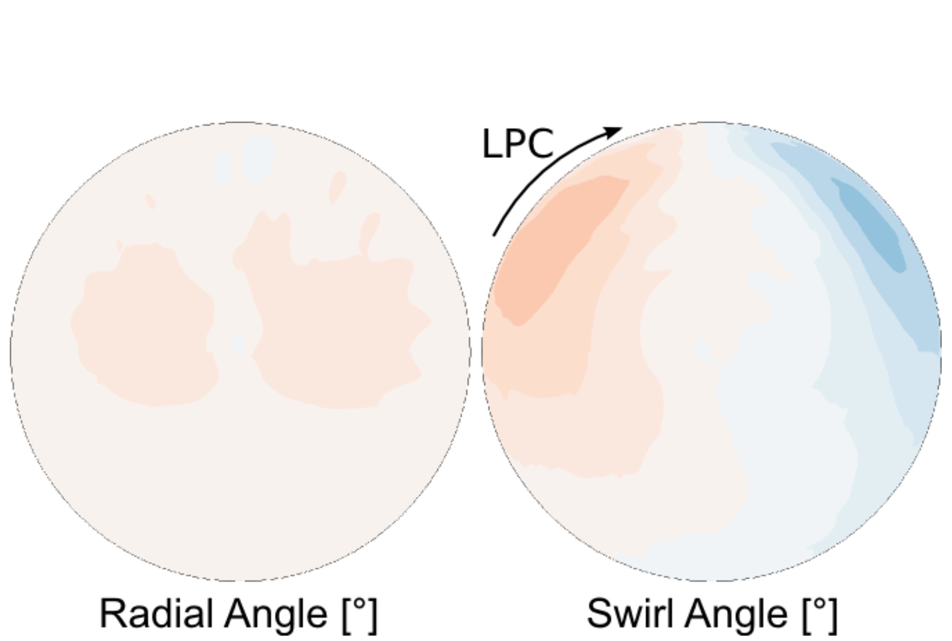
Swirl distortion
Comparing the OP of case 1 with the clean reference case reveals an increase in
Figure 7.
Flow field in cs-6 for isolated swirl distortion (case 1) contour levels according to Figure 5.
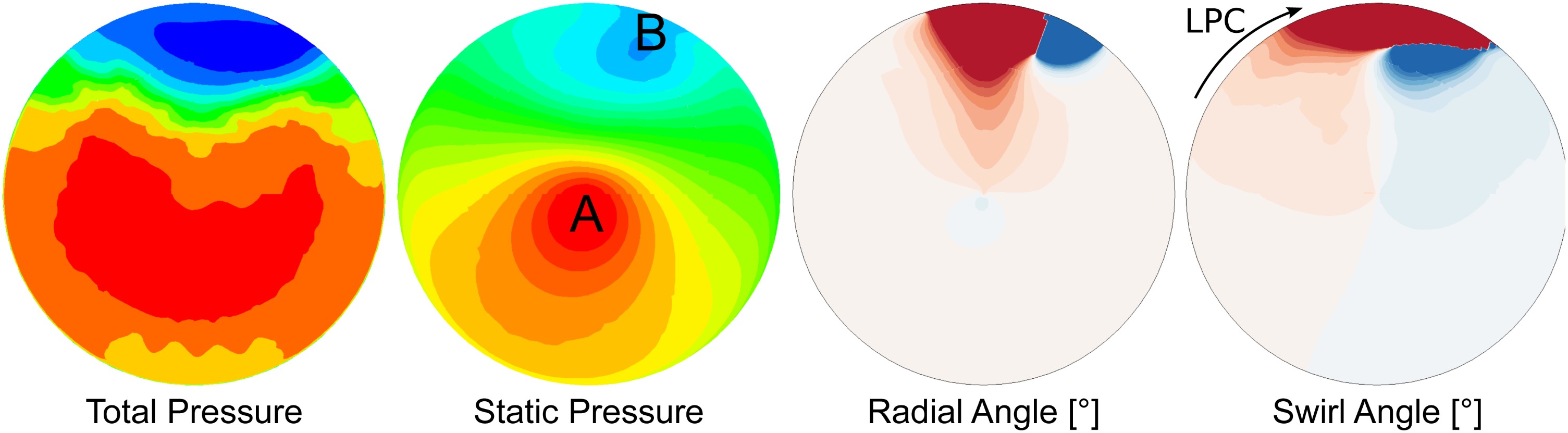
Total pressure distortion
Regarding the OP of case 2, an increase in
Figure 8.
Flow field in cs-6 for isolated total pressure distortion (case 2) contour levels according to Figure 5.
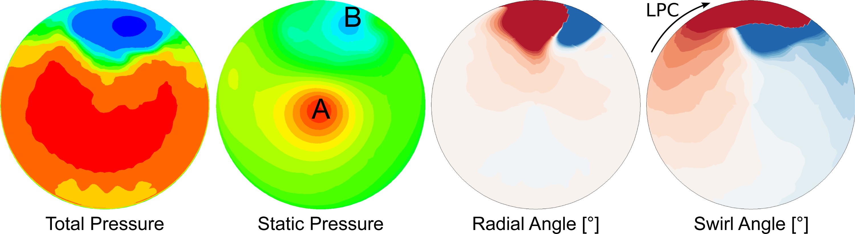
Combined swirl-pressure distortion
The OP of case 3 resembles a superposition of both previous cases: a shift along the speed line in combination with an increased
Figure 9.
Flow field in cs-6 for combined total pressure swirl distortion (case 3) contour levels according to Figure 5.
In the presented calculations, an upstream static pressure field is generated but limited in its upstream propagation by the AIP inlet boundary condition
Coupled intake-compressor simulation
Due to the large simulation domain
Comparison to experimental data
Within the first, contracting part of the intake upstream of cs-3, a similar pressure distribution is observed between both simulation approaches. After cs-3, however, the coupled simulation shows a reduced static pressure along
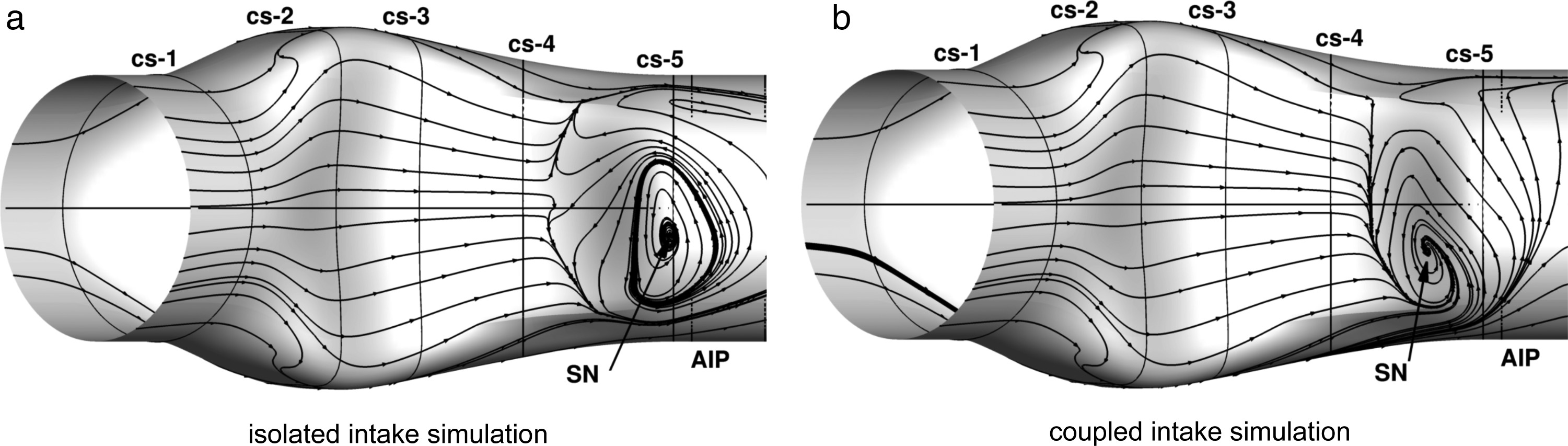
Towards the AIP, the induced static pressure field within the coupled simulation leads to a reproduction of two measured pressure characteristics, which the isolated intake simulation was unable to predict: The local pressure minimum at
Asymmetric AIP flow field
Again, a slight phase shift between the center of the total pressure distortion and the center of the induced static pressure distortion in clockwise (positive rotor rotation) direction is present as it was already seen in cases 2 and 3. It can therefore be identified as a feature of the numerical modeling of the LPC, as it was not measured to that extent in experiments. The asymmetry of the AIP flow field in the coupled simulations is thus composed of two isolated phenomena: First is the already slight asymmetry of the isolated intake flow field (cf. Figure 5) due to inhomogeneous intake inflow. Second is the shift of the induced static pressure distortion in co-rotating direction by the LPC simulation. Both phenomena superpose in case of the coupled simulations and lead to a strong shift of the static pressure distortion, the region of flow separation and the resulting total pressure distortion in circumferential direction.
As the CFD intake flow field shows an increasing asymmetry between cs-3 and AIP in clockwise direction, a further movement of the total pressure distortion is expected towards the rotor inlet plane. The AIP flow field thus shows already a decoupling of the pressure distortions leading to a circumferential extension and thus mitigation of the total pressure distortion.
Conclusions
The flow field in a coupled intake-compressor system was investigated by means of numerical flow simulations. For validation purposes, test data from an extensive measurement campaign of a full size system was available. Two characteristics were of particular interest: The precise prediction of the AIP flow distortion and the intake-compressor interaction. Three simulation approaches were investigated:
An isolated intake simulation requires minor computational resources and calculation time to deliver a converged solution. It is able to reproduce the intake wall pressure field and predicts the occurring flow separation. In case of the investigated duct geometry, however, the AIP lies very close to the separation location. Without the compressor induced static pressure field, the AIP flow distortion predicted by this approach shows backflow and lacks in precision, especially regarding the swirl distortion. The calculated AIP total pressure distortion is stretched in circumferential extent with the minimum total pressure values are underestimated by approximately 5%. Using a two dimensional static pressure outlet boundary condition, the prediction of the flow angles can be improved, but the total pressure distortion remains significantly under predicted.
The influence of the specific inflow distortion components on the operational behavior of the LPC was assessed by means of isolated compressor simulations. An increase in mass flow rate was observed for the investigated swirl distortion, which is not yet fully understood. The influence of the total pressure component of the distortion is comparable to a respective throttling of the compressor and moves the operational point along the speed line but with a further reduction in
Finding the respective operation point for the coupled calculation of intake and compressor is challenging: An adjustment according to the measured intake inflow Mach number leads to a reduced compressor
The under prediction of the s-duct total pressure distortions is a general problem of RANS computations. The special design of the investigated intake geometry, however, with a severe flow separation shortly upstream of the AIP is a very challenging test case for a proper prediction of the AIP flow angles. Using coupled intake-compressor simulations only leads to a slight improvement, as the upstream static pressure field is under predicted by CFD on the one hand and dependent on the incoming total pressure distortion on the other hand. Further investigations will focus on the reasons of the observed unsteadiness of the operation point as well as the asymmetry of the intake flow field. Therefore, additional operation points are simulated. Additionally, the distortion transport through the three stages of the compressor and the decoupling of the specific distortion patterns is of interest.