Describing turbulence anisotropy

Any arbitrary turbulence state can be reconstructed by a linear combination of the three limiting turbulence states, namely: one-component (1C), isotropic two-component (2C), and isotropic (3C). Isotropic 3C turbulence, as the name suggests, forces the anisotropy to be zero, also called “spherical-shape” turbulence. Isotropic 2C turbulence represents a turbulence state in which only two fluctuating components of equal intensity exist (“pancake-shape” turbulence). In contrast, one-component turbulence (1C) is characterized by one fluctuating component which dominates over the other two (e.g., grid turbulence through axisymmetric expansion) and is called “cigar-shape” turbulence. Flows in engineering applications are usually strongly non-equilibrium and anisotropic due to boundaries and high adverse pressure gradients. Turbulence anisotropy can be quantified by the Reynolds stress anisotropy tensor aij, whose incompressible form is given by

Testcase

In this study, the highly loaded LPT profile MTU-T161 described by Gier et al. (2010) has been selected. Non-protected experimental as well as RANS (LEVM) and DNS simulation results were first published by Müller-Schindewolffs et al. (2017). The aerodynamic design point and the geometrical parameters of the LPT profile are given in Table 1.

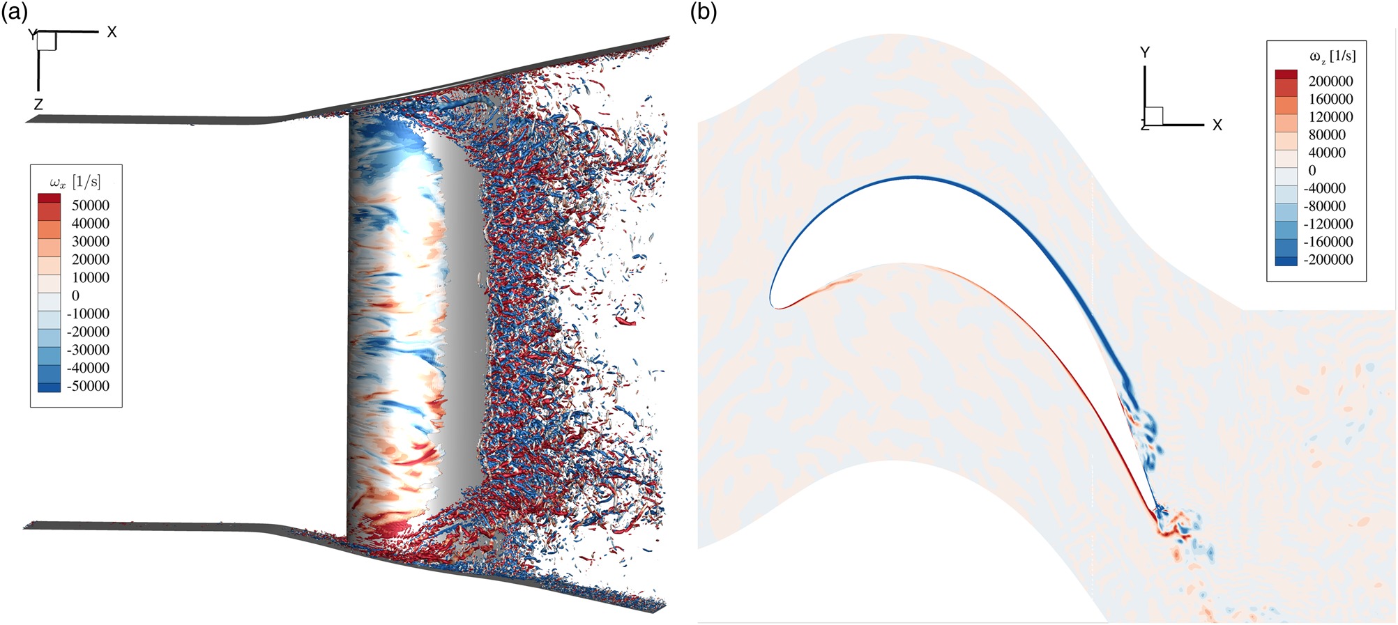
The three-dimensional model of the MTU-T161, including the diverging side walls, is shown in Figure 1a and the blade-to-blade view in Figure 1b. The profile has been investigated experimentally by Entlesberger et al. (2005) at the University of the Armed Forces in Munich. The measurements include inflow turbulence, profile pressure distribution and wake values. The measured freestream turbulence intensity of the cascade tunnel was increased by using a turbulence grid up to 9%, decreasing to almost 3.5% at the leading edge. The experimental results indicate a rapid increase in losses for Reynolds number below 120 × 10³, as the laminar separation bubble on the suction side of the profile grows.

Figure 1.

Instantaneous flow field for the MTU-T161 profile obtained by LES. (a) 3D view of turbulent structures (isosurfaces of λ2 criterion, colored by streamwise component of the vorticity). (b) Blade cut at mid section colored by spanwise component of the vorticity.

Numerical method

RANS (LEVM and DRSM) and LES calculations of the above 3D configuration were conducted using DLR’s TRACE solver for turbomachinery flow simulation. TRACE has been used for LES of LPTS application in the past (Leyh and Morsbach, 2020; Morsbach and Bergmann, 2020). The LES calculations in TRACE solve the filtered compressible Navier-Stokes equations using a second-order accurate, density-based finite volume scheme applying MUSCL reconstruction (van Leer, 1979). LES uses a fraction of 10⁻³ of Roe’s numerical flux (Roe, 1981), which is added to a central flux to avoid odd-even decoupling. The time integration is performed, in this case, using a third-order accurate explicit Runge-Kutta method. The subgrid stresses are computed by the WALE model developed by Nicoud and Ducros (1999).

A one-dimensional characteristic non-reflecting boundary condition implemented by Schlüß et al. (2016) is used at the domain outlet to drive the time- and surface-averaged boundary state towards the prescribed values (static pressure). For the simulation domain inlet, a Riemann boundary condition is applied to set the stagnation pressure, stagnation temperature and flow angles. To reproduce realistic operating conditions, synthetic turbulent fluctuations in the inflow are introduced. The synthetic turbulence generator in TRACE uses the prescribed turbulent length scale and the Reynolds stress tensor components to represent the fluctuation field at the inlet based on superposition of Fourier modes (Shur et al., 2014). These values are adapted from measurements such that the turbulent decay (from simulation inlet to leading edge) matches the experimental decay.

The LES grid consists of 85 × 10⁶ nodes, with a normal wall resolution of y+<1. The values of Δx+ and Δz+ are below 30 and 25 respectively, on the whole suction side. However, beginning at the accelerated laminar boundary layer close to the suction peak up to the trailing edge, the values of Δx+ and Δz+ are below 10, which assure a wall-resolved LES (Tucker, 2014). This is necessary for a detailed analysis of turbulence, especially in the near wall region.

The LES simulation is initialized using the k−ω solution. To avoid averaging over the initial transient phase, recording statistics is started after 10 convective time t_c, which is defined as

with an axial chord length lax=0.06m and an approximate axial velocity at the domain outlet uax,out≈77m/s. The start of the sampling period was chosen by evaluating several convergence criteria, such as acting forces on the blade surface, probe data at several locations, and analyzing the truncated mean-squared error, as described in Bergmann et al. (2022). After the initial transient is washed out, the statistics are accumulated for 40 convective times. This has been shown to be sufficient for a statistical convergence regarding the blade profile and wake values. The simulation has been conducted on a CPU system using Intel Skylake processors with a wall clock time of 336 hours on 1,152 CPUs for 40 convective times.

The steady-state LEVM solution in this work was calculated by applying the k−ω turbulence model developed by Wilcox (1988), with the stagnation-point anomaly fix by Kato and Launder (1993), the γ−ReΘ transition model developed by Langtry and Menter (2009) and a viscous blending technique described in Bode (2018) as an eddy viscosity limiter.

In order to extend the comparison, the hybrid SSG/LRR-ω differential Reynolds stress model developed in the EU-project FLOMANIA (see e.g. Eisfeld and Brodersen (2005) and Eisfeld et al. (2016) coupled with the γ−ReΘ transition model of Langtry and Menter (2009) was used. Contrarily to the linear k−ω turbulence model which uses a constitutive relation to compute the Reynolds stresses based on Boussinesq’s hypothesis, the SSG/LRR-ω full second-moment DRSM solves for each of the six Reynolds stresses a separate transport equation plus an additional transport equation for a variable determining the length scale. The basic idea of the SSG/LRR-ω model is to blend the ϵ-based SSG model (Speziale et al., 1991) for regions of free shear flow with the LLR model (Launder et al., 1975) near walls in the ω-based formulation. The model was chosen because in the solver TRACE only for this RSM a coupling with a transition model is available, which is necessary to capture the transition mechanism, separation and attachment.

Comparison to experiment

Prior to a detailed investigation of the turbulence and anisotropy behaviour, the blade loading and the wake loss are evaluated and compared to the experimental results.

Figure 2a shows the isentropic Mach number (Ma_is) distribution, which is determined by the static pressure, around the profile. The LEVM results match very well with measurements at the leading edge, trailing edge and the aft pressure side. On the suction side, the Ma_is-distribution starts to deviate at x/lax=30%, where the simulation leads to larger Mach number and a shift of the suction peak downstream of the measured peak, from x/lax=60% to 65%. Also the subsequent separation starts later than the measured one, but is much smaller and reattaches well before the trailing edge, at x/lax=90%. The DRSM results are almost identical to the LEVM results. Despite modelling the Reynolds stress separately and taking into account the transition via a transition model, there is no improvement considering the isentropic Mach number distribution. SSG/LRR-ω Reynolds-stress model uses a simple, linear model close to solid walls without any corrections. This might have a negative influence on representing the boundary layer state. In contrast, the LES simulation is in a much better agreement with the measurements, in particular at the suction peak and separation region. A similar situation is shown downstream the cascade at x/lax=1.4, where LES predictions match the measured total pressure loss value very well, whereas the LEVM and DRSM simulations yield a thinner wake with a larger peak value.

Figure 2.

Comparison of averaged quantities of LES, LEVM, DRSM and experiment. (a) Ma_is distribution at 50% span. (b) Total pressure loss coefficient at x/lax=1.4.

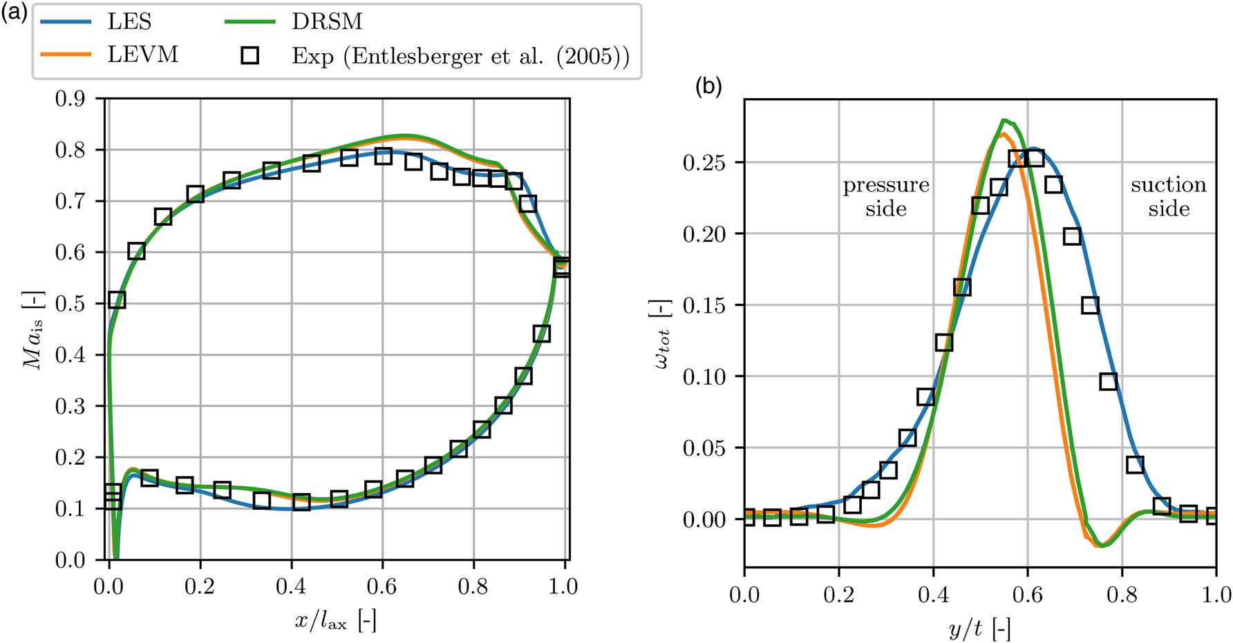
The deficiencies of both RANS models to accurately predict the pressure distribution and the flow loss may be tracked back to the non-adequate reproduction of the turbulence effects in the separation and wake region. Since the separation point is in the laminar state, the turbulence is generated at the outer part of the separation bubble, where strongly anisotropic characteristics are present, as will be shown later. These characteristics are also propagated into the wake. The results of Figure 2 show that even DRSMs (SSG/LRR-ω in particular) have difficulties to capture the transition and separation bubble correctly. Such deficits have also been reported by Eisfeld et al. (2016) and Morsbach (2017). DRSMs offer improvements over the classical LEVMs and EARSMs when turbulence structure is considered. However, these improvements do not always extend to the mean flow quantities. Since the prediction of the boundary layer state and the modeling of the Reynolds stresses are some of the key parameters, the following sections of this paper will focus on a more detailed analysis based on anisotropy and the share of Reynolds stresses in the suction side boundary layer.

Separation and transition to turbulence

It has been shown Coull and Hodson (2011) that two mechanisms dominate in LPT applications under elevated free stream turbulence (FST) conditions (2%−3% in the free stream and outer boundary layer in the current case). Firstly, the incoming turbulence interacts directly with Kelvin-Helmholtz (KH) rollers, leading to spanwise disturbances and subsequent breakdown. Secondly, the incoming turbulence accelerates the transition by creating turbulence spots in the initial part of the boundary layer. The transition is triggered by the development of the so-called Klebanoff streaks and a destabilized separated shear layer. Several authors argue that the KH instability plays a dominant role in the transition process of separation bubbles, whereas other experimental studies claim the Tollmien-Schlichting waves to be more significant (Roberts and Yaras, 2003; Rist et al., 2004; Volino, 2010; Yang, 2011).

To facilitate further discussion, a body-fitted coordinate system is introduced for the suction side region of the profile, with coordinate s starting from leading edge running to trailing edge and coordinate t representing the wall normal direction (Figure 3a). As such, we performed a transformation to the new coordinates for the region of interest on the suction side. In this area, velocities and Reynolds stresses are transformed to the new coordinate system where the indices 1, 2 and 3 indicate the wall parallel, wall normal and spanwise direction. t_max characterizes the edge of the wall normal coordinate t.

Figure 3.

Turbulence in the blade passage obtained by LES. (a) Turbulent kinetic energy (logarithmic scale). (b) Componentality of Reynolds stress anisotropy tensor.

The suction side boundary layer around the MTU-T161 is characterized by the separation-induced transition mode. As shown in Figure 3a, the suction side boundary layer separates at around x/lax=0.61 (region 1①). As a consequence, the transition is triggered and completed in the aft section of the suction side, reaching a full turbulent state. This is supported by the maximum values of turbulent kinetic energy (TKE) shown at the bottom of Figure 3a (region 2②). The maximum shear line (max(∂u1/∂t)) right above the separation bubble highlights the trajectory of the high TKE values. For the same geometry and operating point, Müller-Schindewolffs et al. (2017) showed that the laminar separation bubble causes an intensive Kelvin–Helmholtz instability, leading to the transition and the reattachment of the bubble.Nevertheless, the main focus of the current work is not to discuss the prevailing transition mechanism in detail, but rather to demonstrate and analyze the turbulence anisotropy behavior of the suction side boundary layer (including separation bubble, shear layer and reattachment regions).

Turbulence anisotropy

To get a better overall understanding of the turbulence state, Figure 3b shows the componentality contours in blade-to-blade view. To do this, the methodology of Emory and Iaccarino (2014) is used, by mapping the weights Cic of the barycentric map to the RGB channels. The inflow is characterized by moderate isotropic 3C incoming turbulence, which is consistent with the applied turbulent boundary conditions (region 3③). In freestream, the isotropic turbulence state enters the passage until it reaches the acceleration region, promoting a shift to 2C turbulence indicated by the change from blue to green color in Figure 3b (region 4④). In this region, spanwise and pitchwise fluctuations make an almost equal contribution to the turbulence level. The origin of the 2C turbulence state can be mainly traced back to the velocity gradient governing in the passage flow (Behre, 2019). Following a streamline in the middle of the passage, as shown in the Figure 3b at the top, the flow experiences a significant velocity gradient along and normal to the streamline. The high pitchwise gradient promotes the production of turbulent energy in pitchwise direction. The energy is partially redistributed to the other two components. The streamwise gradient, in an identical fashion, causes a partially redistribution to the pitchwise and spanwise component, as shown by Behre et al. (2021).

The near wall area of the profile is dominated by 1C turbulent state, in this case streamwise Reynolds stress. The 1C layer (red color) spans from near leading edge to the separation point. After the flow starts to separate, the prominent 1C turbulence state is stretched along the line, indicating the maximum shear above the reverse flow region.

The second region of interest is the 2C area directly above the 1C layer next to the wall (region 5⑤). The 2C layer follows the same path as the 1C near the wall. The origin of this phenomena can be traced back to the redistribution effect of the incoming free stream 3C isotropic background turbulence at the stagnation point of the leading edge. As has been shown by Xiong and Lele (2007), the wall normal fluctuations at the stagnation point decrease close to the wall due to the non-penetration condition. The energy of the wall normal fluctuations is transferred to the other two components, creating a 2C state in the vicinity of the stagnation point. This state is convected downstream, with the mean flow tangential to the blade surface, causing the 2C layer (green color). Turbulence entrainment from the free-stream into the laminar boundary layer patch undergoes the same redistribution of the wall-normal component, together with the turbulence damping. As a result, the 2C layer is still present along the complete laminar boundary layer part.

In the separated region (s/smax=0.61), the 2C turbulence is dominant close to the wall, while the turbulence away from the wall becomes isotropic. The area inside the separation bubble is characterized by 2C and 3C turbulence, with 3C turbulence being more present from s/smax=0.8 (region 6⑥).

In summary, Figure 3b demonstrates the complexity of the investigated flow and indicates that nearly all possible states of turbulence occur in different regions of the suction side. At the same time, this explains to some extent, why most of the RANS eddy viscosity turbulence models (e.g. standard k−ω), fail to predict complex separated flows. However, the detailed characterization of the turbulence is the key element for development of appropriate RANS model extensions.

After looking at the composition of the Reynolds stress anisotropy tensor of the flow, subsequent figures illustrate relevant turbulence states in respect of the contribution of the different fluctuating components.

Figure 4 shows contour plots of the normal and shear Reynolds stresses, normalized by the mean outlet velocity (u_ref). Superimposed are the inflection line (u1/uref=0) and maximum shear line. In order to discern separation and reattachment points, the skin friction coefficient cf - calculated on averaged statistic samples - is also plotted in Figure 4a. Following these plots, the boundary layer separates at around s/smax=0.61 and reattaches at around s/smax=0.93. This is confirmed by the skin friction coefficient, crossing zero for the first time and reaching positive values in the aft section.

Figure 4.

Skin friction coefficient cf and Reynolds stress components (with logarithmic scale) along the suction side obtained by LES. (a) Skin friction coefficient cf. (b) streamwise Reynolds stress component u1′u1′¯/uref2. (c) wall normal Reynolds stress component u2′u2′¯/uref2. (d) spanwise Reynolds stress component u3′u3′¯/uref2. (e) shear Reynolds stress component −u1′u2′¯/uref2.

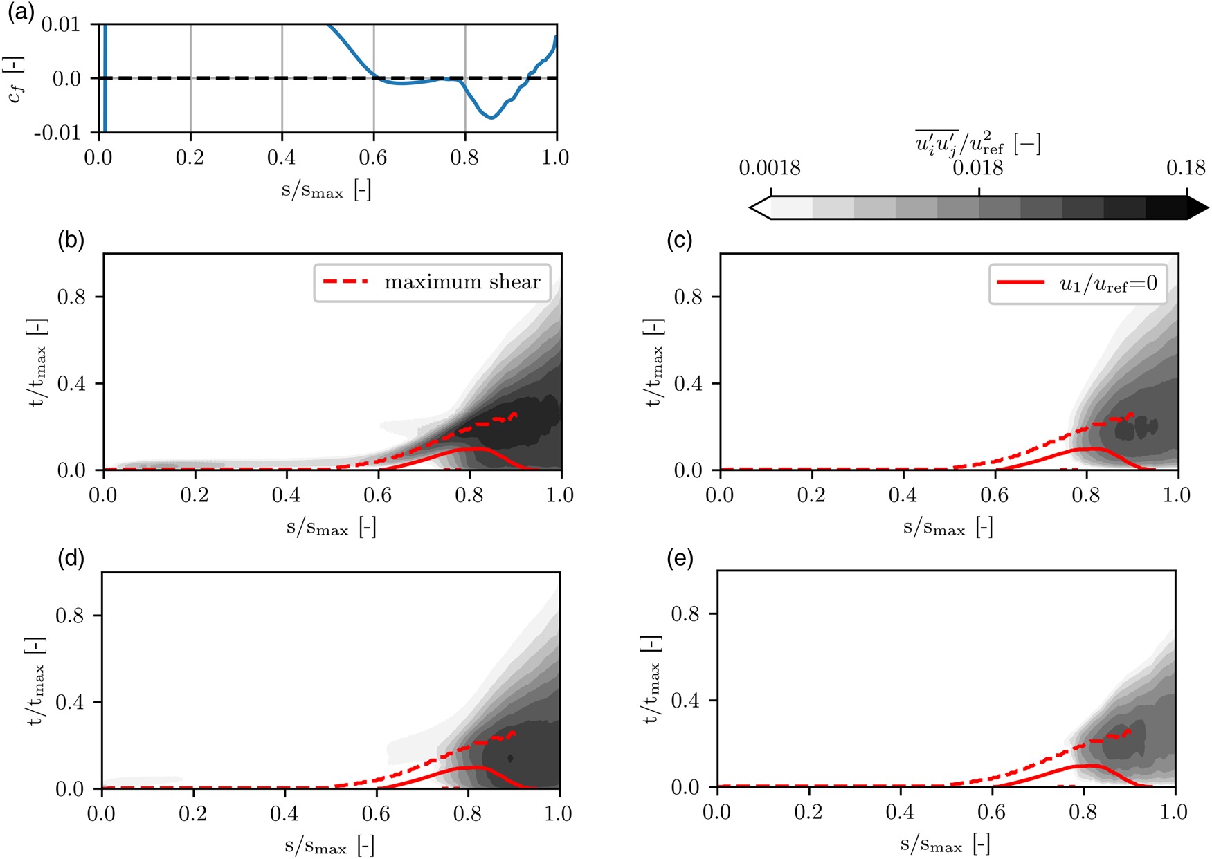
One should note that identifying a reattachment point or line, based on the skin friction plot, is justified for a steady laminar separation bubble. Whereas in transitional and turbulent separation bubbles, the instantaneous flow field is highly unsteady and varies continuously over time. The definition of a reattachment point could therefore be misleading. Here, the definition is based on the time-averaged velocity distribution. Looking at the streamwise Reynolds stress component u1′u1′¯ (Figure 4b), a continuous amplification along the max shear line can be observed. This reaches a maximum value of 12% around s/smax=0.86, while propagating highly turbulent flow towards the wall. This effect is in line with the maximum negative value of the skin friction coefficient and high turbulent kinetic energy (Figure 3a). The high levels of the streamwise velocity stresses can be traced back to the streamwise streaks (pre-transitional Klebanoff modes) generated in the upstream laminar boundary layer. These streaks become unstable and end up generating turbulent spots in the shear layer. The streamwise component has the highest contribution among the Reynolds stress components and shows a steep growth from leading edge, which is perfectly in line with the 1C turbulence layer shown in Figure 3b.

Both wall normal u2′u2′¯ and spanwise u3′u3′¯ Reynolds stress components (Figure 4c and 4d, respectively) are negligible upstream of the separation bubble and start to grow simultaneously, at arounds/smax=0.8. Spanwise fluctuations are the second important contribution regarding the intensity. In the rear part of the separation bubble, the Reynolds shear stress u1′u2′¯ (Figure 4e)reaches almost the same value as the wall normal Reynolds stress. This is strongly related to the amplification and saturation of the instabilities and indicates the fully turbulent state. The maximum value of fluctuations is reached where large-scale vortex shedding occurs (as a consequence of the shear layer roll-up) and represents the strength of the large-scale turbulence in moving freestream fluid towards the surface.

Wall normal profiles of turbulence

After investigating the streamwise evolution of the anisotopy and Reynolds stresses, the following figures present with the Reynolds stress distribution perpendicular to the wall. As in Figure 3b, to get a better overall understanding of the turbulence state, the componentality contours are visualized by mapping the weights Cic of the barycentric map to the RGB channels via the barycentric map. To this end, four relevant axial positions on the suction side surface are selected (marked lines in Figure 3a top left). Additionally, the turbulence anisotropy state is plotted as a barycentric RGB map. It should be noted that the ranges of x and y axis are plotted independently in each sub figure. This is due to a better visualization of the fluctuations in the boundary layer. Since the fluctuations and the corresponding turbulence anisotropic behavior differ considerably depending on the boundary layer state.

Starting from the front part of the suction side in Figure 5a, in which the flow accelerates and a laminar boundary layer exists, a mixture of 1C and 2C isotropic turbulence state is observed in near wall area (y+<20). Moving further towards the outer layer of the boundary layer, the spanwise contribution becomes more prominent, moving more towards isotropic 2C turbulent state, as seen in Figure 3b. The turbulence state outside the boundary layer is governed by isotropic 3C. This pattern is maintained, after passing the suction peak (maximum of Mais on the suction side) at s/smax=0.3 and reaching the separation bubble at s/smax=0.6 (Figure 5b). There is a difference in the free-stream flow, compared to the axial positions before s/smax=0.3, which is the result of the passage flow acceleration (see the discussion of Figure 3b). The streamwise component shows two distinct peaks and the near wall region (y+<5) shows a isotropic 2C manner. The turbulence anisotropy state becomes more complex proceeding further into the separated region (Figure 5c). At this streamwise position, the streamwise fluctuation starts to grow rapidly (Figure 4). At the same time, in the region close to the wall (y+<5), there is a 2C anisotropy state, which is not the case in the upstream laminar region of the boundary layer.

Figure 5.

Reynolds stresses (lines) and the corresponding componentality of Reynolds stress anisotropy tensor (colorbars) along wall normal lines at four defined streamwise positions as in Figure 3a obtained by LES. (a) s/s_max = 0.3. (b) s/s_max = 0.6. (c) s/s_max = 0.75. (d) s/s_max = 0.85.

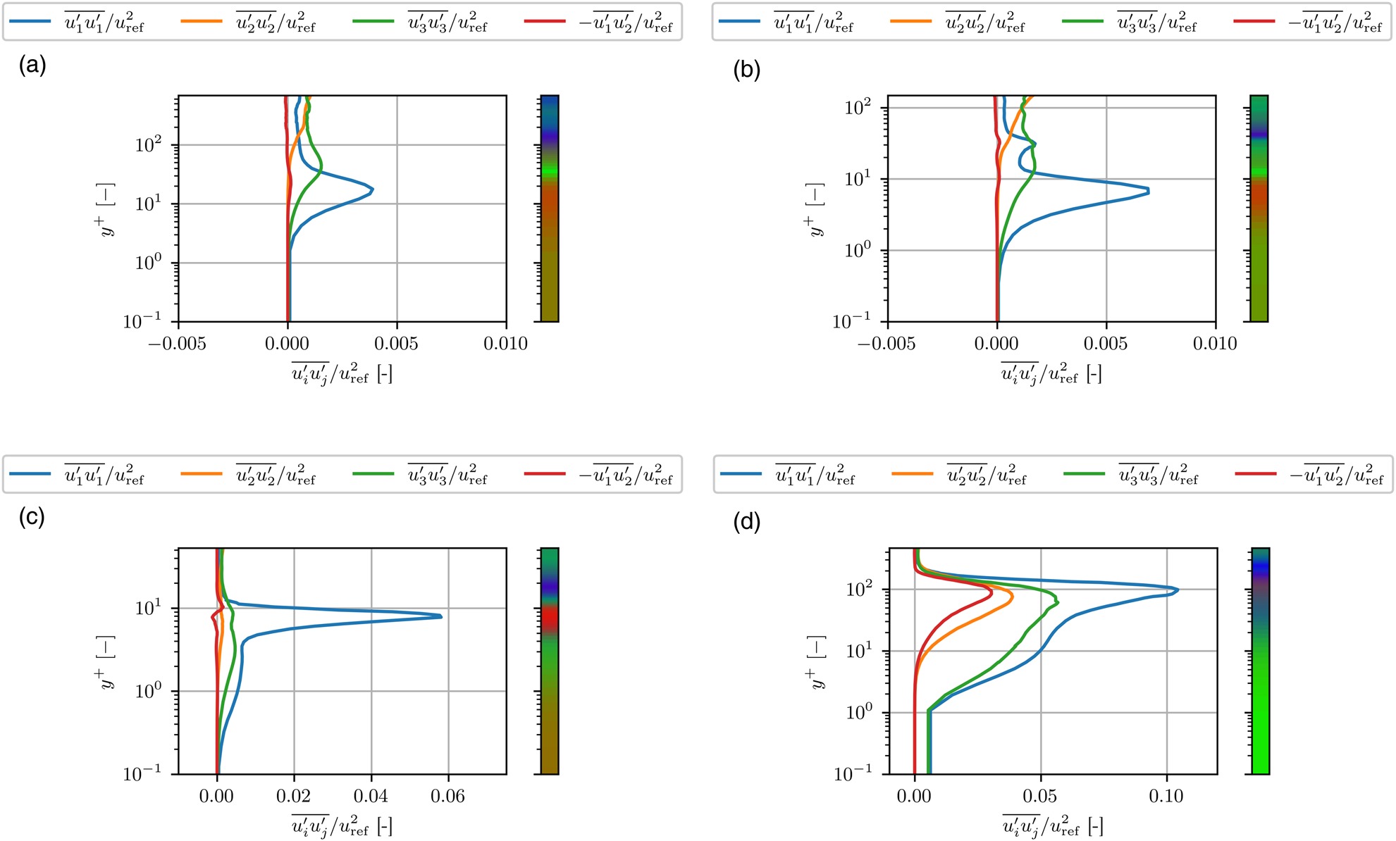
Moving further downstream (Figure 5d), all Reynolds stress components increase and reach their maximum level at y+≈100. In addition to the normal Reynolds stresses (u1′u1′¯,u2′u2′¯ and u3′u3′¯), the shear stress u1′u2′¯ also increases, which is a clear indication of the momentum and energy exchange between all Reynolds stress components. Equally important is the presence and influence of a detached shear layer itself. The separated boundary layer transports the turbulence above the separation bubble and results in high Reynolds shear stresses and turbulence production. This is consistent with the findings in Figure 4. Obviously, there is a lag of the shear stress component when compared to the normal components. While the normal components are present at all positions (in a different manner and amount), the shear stress component is only persent at the last position, where the transition process towards the fully turbulent state is completely finished.

Moving towards the edge of the boundary layer, the 2C turbulence becomes 1C in a thin region with dominant streamwise component, but is quickly changing to 3C state at the boundary layer edge. As mentioned before, the layer further above changes again to 2C state, due to flow acceleration and turning inside the turbine passage.

Comparison to RANS

Figure 6 demonstrates the difference in the prediction of Reynolds stress components between RANS (both LEVM and DRSM) and LES at s/smax=0.85. It should be noted that the plot of each numerical model is shown separately, since the fluctuations and the corresponding turbulence anisotropic behavior differ considerably depending on the boundary layer state in RANS and LES. In contrast to LES, the LEVM result in Figure 6a indicates isotropic 3C turbulence throughout the whole separation bubble. This is confirmed by similar values for normal Reynolds stresses (u1′u1′¯≈u2′u2′¯≈u3′¯u3′). Further, the magnitude of the LEVM predicted normal stresses and the corresponding turbulent kinetic energy is much smaller than the corresponding LES predictions. Similar results are reported by Müller-Schindewolffs et al. (2017) and Pichler et al. (2015) for such applications. Looking at the shear stress, similar behaviour can be observed for the LEVM and LES, that means the shear stress is smaller and lags behind the normal stresses. The DRSM is able to reproduce the correct anisotropic behavior only to some extend. Especially the two component turbulence state close to the wall is not captured by the SSG/LRR-ω model. Nevertheless at y+≈40, the DRSM results show, unlike LEVM, a better trend regarding the Reynolds stress contributions. At this wall normal position the DRSM predicts different normal and shear Reynolds stress contributions (u1′u1′¯>u3′¯u3′>u2′u2′¯), which resembles the distribution of LES. The magnitude of the predicted normal and shear stresses and the corresponding turbulent kinetic energy by the DRSM are weaker than predicted by LES.

Figure 6.

Comparison of Reynolds stresses (lines) and the corresponding componentality of Reynolds stress anisotropy tensor (colorbars) between (a) LEVM, (b) DRSM and (c) LES at s/s_max= 0.85.

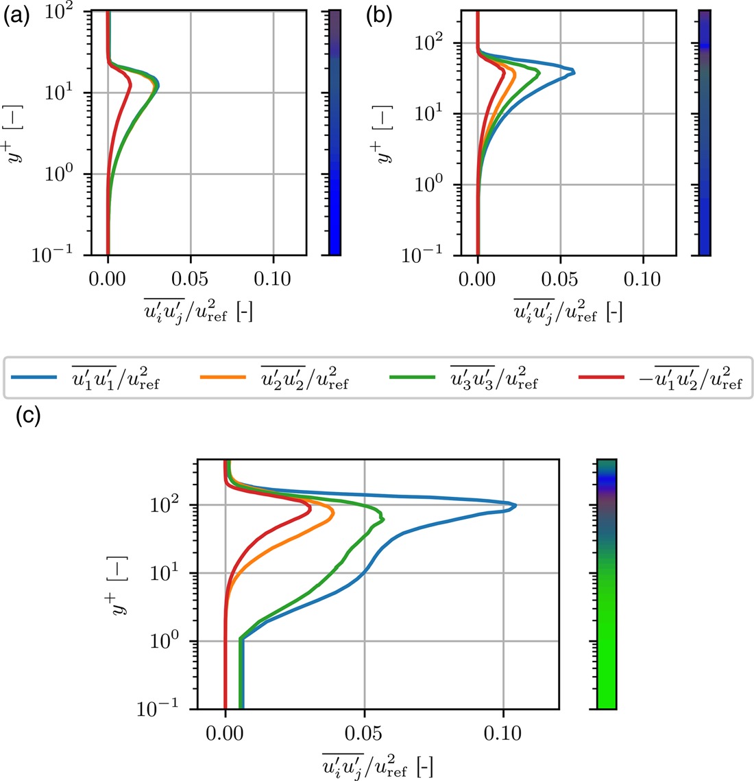
The numerical results show that the underestimation of Reynolds stress is a significant factor in the unsatisfactory prediction of separation. These results emphasize the need to improve the prediction of reverse-flow speed in separation bubbles by LEVMs and DRSMs.

Acronyms

Latin symbols

Greek symbols