Research object

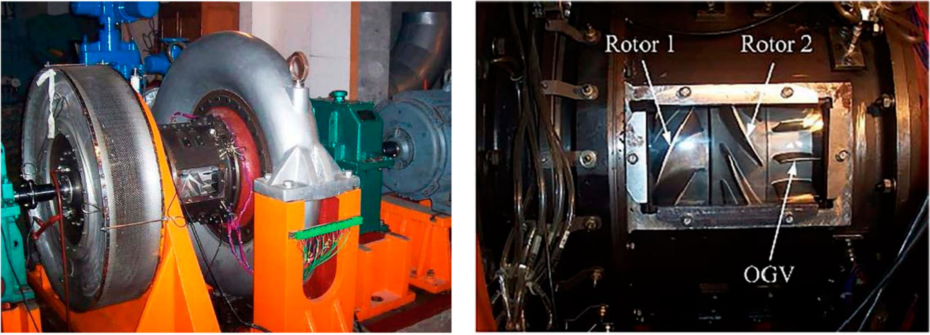
The subject of this study is a two-stage counter-rotating axial compressor, as shown in Figure 1. The compressor consists of four blade rows, namely: inlet guide vanes (IGV), front rotor (R1), rear rotor (R2), and outlet guide vanes (OGV). The blade number for the inlet guide vanes and the outlet guide vanes are 22 and 32, respectively. Operating at the design flow rate of 6.4 kg/s, the compressor has a total pressure ratio of 1.22 and an isentropic efficiency of 89%. Other key design parameters of the CRAC are presented in Table 1.

Figure 1.

Physical picture of the CRAC test bench.

Numerical methods

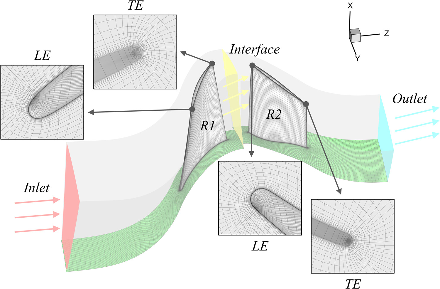
Given that the focus of this study is on the stall evolution process and mechanisms of CRAC, with particular emphasis on the aerodynamic stability and flow field characteristics in the tip region, only the two rows of rotors were simulated in the numerical computations. Additionally, the blade number of R1 was increased from 19 to 20 through a computational domain scaling method, while ensuring that the blade pitch remained unchanged. The mesh was automatically generated using NUMECA/Autogrid5, as depicted in Figure 2. The inlet and outlet computational domains are H-type grids, while the inter-rotor tip clearances are discretized using O4H-type grids. The tip clearances themselves are meshed with butterfly grid topology, with a radial node count of 25. The height of the first grid layer adjacent to the solid walls is set to 0.5 µm to ensure that y+ is less than 2.0, which satisfies the requirements for the Spalart-Allmaras turbulence model used in this paper. The research group had previously conducted a grid independence study (Guo et al., 2023), which determined that when the grid number for a single blade passage was approximately 1.68 million, the computational results no longer exhibited significant changes with further increases in grid number. Therefore, in this study, the numerical calculations for a single passage adopt this grid configuration. According to the research by Pullan et al. (2015), in the numerical computation process, when the circumferential coverage of the computational domain exceeds 1/4 of the whole annulus passage, the computational results can essentially capture the inception of stall cells in the stall process. Therefore, this paper sets the total number of blade passages in the numerical computation to 5 to meet the circumferential coverage requirement.

Figure 2.

Schematic diagram of computational domain.

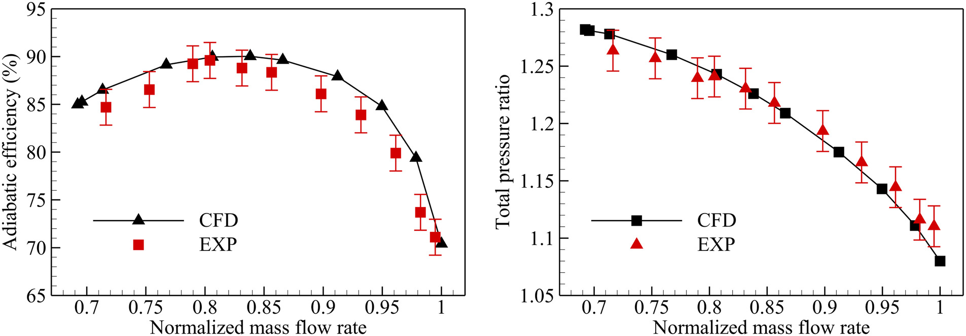
This paper employs NUMECA/Fine Turbo for numerical simulation, utilizing the finite volume method in conjunction with the Spalart-Allmaras turbulence model to solve the three-dimensional Reynolds-averaged Navier-Stokes equations in a relative coordinate system. The spatial discretization is performed using a second-order accurate central difference scheme. In the steady calculations, the time term is iteratively solved using the fourth-order Runge-Kutta method, and data is transferred across the interface of the two rotors using the circumferential conservation method. In the unsteady calculations, a dual-time stepping implicit iteration method is used for solving the equations, and data is transferred across the interface of the two rotors using the sliding mesh interface method. The physical time is set to 80 steps per blade passage, with 30 pseudo-time iterations performed for each physical time step (Guo et al., 2023). The results from the steady calculations are used as the initial flow field for the unsteady calculations. The boundary conditions are set as follows: the inlet is specified with total temperature and total pressure, and the flow direction is axial. The outlet is set to an average static pressure, and the solid walls are designated as smooth and adiabatic. The overall characteristic curve of the compressor is obtained by varying the average static pressure at the compressor outlet. As the compressor approaches stall, to more accurately determine the stall boundary, the bisection method is employed to alter the outlet average static pressure, with the minimum step size set to 25 Pa. At the design rotating speed, the numerical calculations were compared with experimental results to verify the reliability of the numerical method. Figure 3 presents a comparison between numerical calculations and experiments. The mass flow rate in Figure 3 is normalized based on the blockage mass flow rate calculated by CFD. It can be observed that there is a good agreement between numerical simulations and experimental data, indicating that the numerical method employed in this paper possesses a reasonably reliable predictive accuracy.

Figure 3.

Comparison of overall characteristics between numerical and experimental results.

Overall performance and stall evolution analysis of CRAC

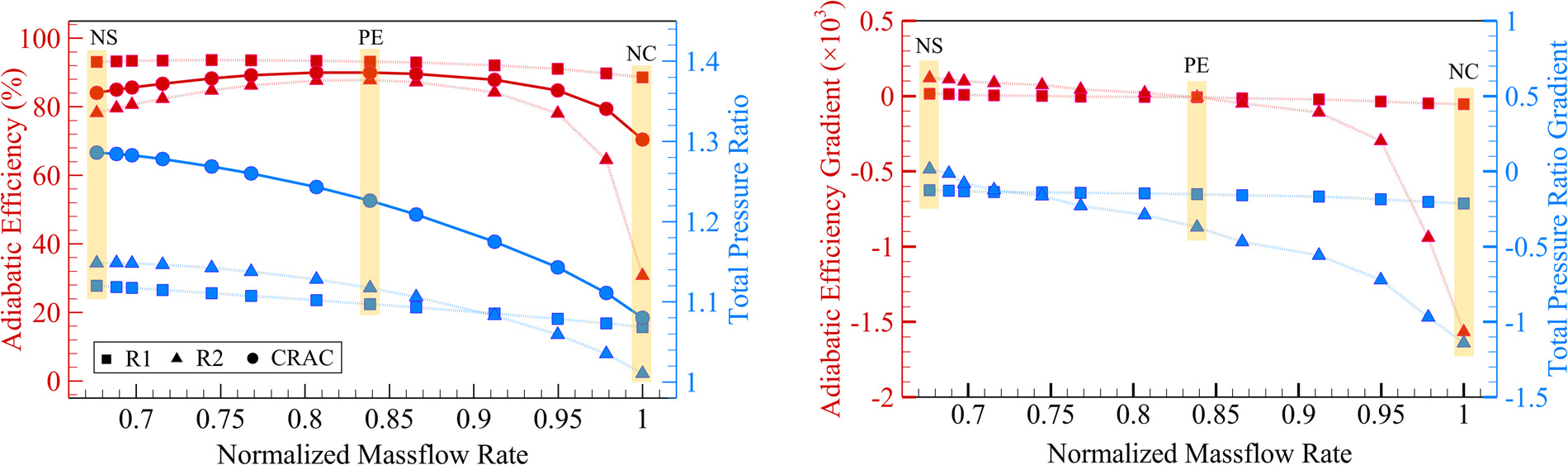
This paper first investigates the stall evolution process of the CRAC. Figure 4 presents the characteristic curves of the isentropic efficiency and total pressure ratio for the CRAC, R1, and R2, where NS, PE, and NC denote the near-stall, peak efficiency, and near-choke conditions respectively. One can see that the isentropic efficiency of R1 is higher than that of R2 within the whole operating flow range. However, the pressure rise capability of R1 is weaker than that of R2, except near NC. Moreover, Figure 4 (right) demonstrates that R1 is less sensitive to flow variations compared to R2, which implies that the overall characteristic variations of the CRAC are primarily dominated by R2. As the CRAC operating state shifts from PE to NS, the decrease in isentropic efficiency is mainly due to the efficiency drop of R2, and the deceleration of the total pressure ratio increase is also attributed to the reduced pressure rise of R2. Therefore, the stall of the CRAC is more likely to be initiated by R2.

Figure 4.

Comparison of overall characteristic of CRAC.

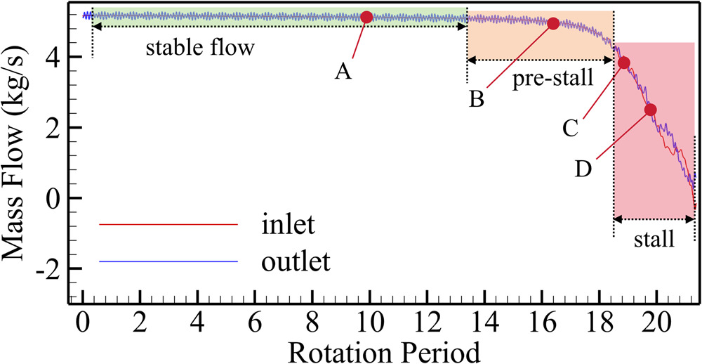
Subsequently, the stall process of the compressor is further analyzed using the results of unsteady calculations. Figure 5 presents the variation curves of the inlet and outlet massflow rates of CRAC during the stall process. As illustrated in the figure, the entire stall process is divided into three distinct stages based on the evolution of the flow rate: stable flow, pre-stall and stall stage. The stable flow stage is defined as the period where the flow rate remains stable. The pre-stall stage is characterized by the onset of flow rate decline. The stall stage is identified by a significant decrease in the flow rate. One moment from the stable flow stage and one from the pre-stall stage were selected for analysis, while two moments were chosen from the stall stage. These four moments represent four typical flow characteristic moments during the complete stall process (stable flow, stall inception, stall development, and deep stall), and they are denoted chronologically as A, B, C, and D. Figure 6 presents the vortex structures of the CRAC for the four moments from A to D, utilizing the third-generation vortex identification method proposed by Liu et al., known as the Liutex-Omega method (Liu et al, 2019, 2020). The method identifies vortex regions based on the relative vortex intensity ωR and employs the absolute vortex intensity R for vortex coloring. Unlike conventional vortex identification methods such as Q, λ2, Δ, λci, and other second-generation vortex identification techniques, the Liutex-Omega method effectively eliminates the contamination of vortex identification by shear and stretching compression. It offers clear physical significance, ease of implementation, normalization, the ability to capture both strong and weak vortices simultaneously, and the advantage of not requiring significant threshold adjustments. Therefore, using the Liutex-Omega method to identify the vortex structures during the stall process ensures that the vortex structures are accurately depicted, preventing interference in the flow field analysis that could arise from ambiguous vortex structures.

Figure 5.

Variations in inlet and outlet massflow rates during the stall process of CRAC.

Figure 6.

Evolution of vortex structures of CRAC (ω_R = 0.55).

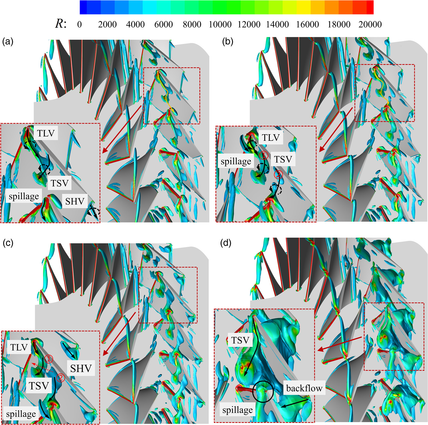
The results depicted in Figure 6 indicate that during the stall process of compressor, the vortex structures of R1 do not undergo significant changes. Moreover, the stall inception and the rotating stall phenomena are predominantly concentrated in R2. Therefore, by analyzing R2, a relatively comprehensive description of the non-stationary phenomena during the stall process can be obtained. Consequently, this paper only focuses on a detailed analysis of the evolution of the vortex structures in R2. At the moment A, which corresponds to the stable flow condition, the main vortices in the tip region of R2 include the tip leakage vortex (TLV), the tip secondary vortex (TSV) (Zhang et al., 2022), and the shedding vortex (SHV). As the TSV moves to the adjacent blade, it gradually disintegrates and dissipates. The remaining segments with higher intensity do not dissipate but instead collide with the LE of the adjacent blade, inducing the occurrence of LE spillage. After several rotation periods at the moment B, which marks the stall inception, two TSVs emerged at the tip of R2. TSV① moved upstream, while TSV② migrated towards the adjacent blade and collided with its leading edge. A comparison of the orange solid lines in Figure 6a and b indicates that at moment B, the fluctuation of the LE vortices at the tip of R2 is more intense, and the unsteadiness of the vortex structures is enhanced. After three rotation periods at the moment C, the formation positions of the two TSVs have both further shifted upstream. TSV① compressed the coverage space of the TLV and suppressed the generation of the TLV, while the interference of TSV② with the adjacent blade intensified, leading to aggravated blockage at the tip leading edge, increased backflow within the tip passage, and the compressor massflow rate begins to rapidly decrease. Simultaneously, at the trailing edge (TE) of the suction surface near the tip, the volume of SHV increased and its intensity is enhanced, further exacerbating the blockage at the TE. After one rotation period at the moment D, the compressor massflow rate rapidly decreases. The TSV completely suppressed the generation of the TLV, and the spillage almost entirely covered the tip leading edge.

The study outlined above of the stall process demonstrates that the TSV gradually moves forward with the reduction of flow rate then interfered and collided with the leading edge of the adjacent blade. The collision induces periodic excitation and progressively enhances the volume and intensity of the LE spillage. Throughout this process, the flow capacity in the tip region gradually diminishes, ultimately leading to a deep stall in the compressor. In contrast to the conclusions drawn from conventional unsteady methods cited in (Gao et al., 2015; Chen et al., 2019; Mao et al., 2019), this study reveals that the breakdown of the TLV and the emergence of LE spillage are not the causes of stall, but rather flow characteristics that appear in the blade LE region imminently before stall. Weichert also arrived at a similar conclusion in his experimental study on the stall inception in axial flow rotors (Weichert, 2012). However, the analysis presented above still does not provide an explanation for the mechanism of TSV generation or the reasons for its forward movement.

In the existing public literature, Wu et al. (2012a,b) in their research on the stall inception in a subsonic compressor, found that the tip separation vortex forms from the interaction of low-energy fluid from blade tip leakage with incoming flow and the breakdown of the leakage vortex. The tip separation vortex which is also referred to as the tip secondary vortex and back flow vortex — essentially similar vortex phenomena but with different names in various literatures. This periodic self-sustaining unsteady flow phenomenon leads to the occurrence of stall spike in the compressor. Chen et al. (2017) investigated the flow structure of an axial compressor rotor at the stall inception. Their study indicated that the occurrence of rotating stall and rotating instability is associated with the development and circumferential propagation of back flow vortex and their unsteady interaction with adjacent blades. Other public literature on the study of TSV tends to focus on the causes for TSV generation and their impact on the stability of compressors. To date, there is no literature analyzing the mechanism of TSV forward movement. Therefore, further exploration is needed to understand the evolutionary mechanism of TSV during the stall inception.

Analysis of stall evolutionrom the perspective of RVMD technique

The analysis in the previous section was limited to a few representative instantaneous flow fields and could not fully describe the entire stall inception process. To further extract the unsteady characteristics of the complete stall process from the data, this section analyzes the space-time evolution of the R2 tip flow field, a key indicator of stall information. Given that axial velocity Vz is the most direct indicator of flow blockage, this study uses the RVMD technique to analyze the 2D axial velocity field at 99% blade height of R2. The analysis decomposes the axial velocity field data from the 10th to 20th rotation periods. In this context, the space-time field data q(x, t) ∈ R^m×n is considered, where each column vector of q(x, t) represents flow parameters at a specific time, with m denoting the number of spatial nodes and n representing the number of temporal nodes.

The RVMD technique is capable of extracting a fixed number of modal information from space-time field data, thereby simplifying the unsteady flow field. The mode decomposition process is as follows. Firstly, multidimensional space-time field data q(x, t) is acquired. In this study, the CRAC data dimensions are m = 44,845 and n = 4,000. In order to reduce computation time, we use SVD to preprocess the data and reduce its spatial dimension. Subsequently, a series of triplet data points (with a total number of K) is identified, namely the RVMD modes:

In the equation, ψk(x) represents the spatial modes, ck(t) denotes the time-evolution coefficients, and ωk is the central frequency of the time-evolution coefficients. The triplet is the solution to the following optimization problem:

The optimization problem is equivalent in the frequency domain to:

The problem is solved using block coordinate descent algorithm. First, the modes, time coefficients, and central frequencies are initialized. Subsequently, the RVMD modes are obtained through multiple iterations. For detailed calculation procedures, one can refer to literature (Liao et al., 2023). Since this paper focuses on frequencies of the same order of magnitude as blade passing frequency (BPF) and low-frequency fluctuations associated with stall, the central frequencies are initialized uniformly across the 0 to 4 BPF range. This approach ensures rapid convergence to the frequencies of interest. Similarly to the VMD method, computing RVMD modes requires manually inputting the empirical filter parameter α and the number of decomposition modes K. This paper determines these two empirical parameters based on the RVMD decomposition of the stall process in the CRAC. Figure 7 presents the spatially averaged PSD across various stages of the stall process. The characteristic frequency bands, representing the main structures of the stall process and targets for RVMD modal identification, are highlighted in gray. The filter parameter α and the number of decomposition modes K should be chosen such that the RVMD modes encompass the aforementioned characteristics.

Figure 7.

Spatially averaged PSD at each stage of stall process.

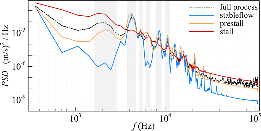
Figure 8 illustrates the variation of the central frequencies of the RVMD modes with respect to the filter parameter α and the number of decomposition modes K. In Figure 8a, K is fixed at 20, while in Figure 8b, α is fixed at 10⁶. The results depicted in the figure show that the filter parameter α has a significant impact on the central frequencies of the decomposed modes. In this scenario, the choice of the filter parameter α plays a crucial role in the performance of the RVMD technique. When α is set less than 10⁵, the decomposition tends to capture predominantly low-frequency modes, which may not be sufficient for capturing the high-frequency characteristics that are often critical in the analysis of complex flow phenomena such as stall. This limitation can lead to a decomposition that is more likely to POD, where each mode contains a broad range of frequencies rather than being representative of specific flow characteristics. When α exceeds 10⁶ the frequency concentration of the decomposed modes begins to decrease significantly. According to the narrowband constraint theory of RVMD, an increase in α can cause each frequency band of RVMD mode to be more concentrated around the central frequency. However, the increased concentration of frequency bands due to the increase in α makes the decomposition effect of RVMD more similar to DMD, with its ability to characterize non-stationary states gradually diminishing. Therefore, α must be large enough to ensure that each mode contains only one characteristic frequency, yet small enough to guarantee that RVMD can represent non-stationary characteristics. The results in the figure also demonstrate that the number of decomposition modes K has a significant impact on the central frequencies of the RVMD modes. When K is less than 16, the decomposition modes fail to encompass all the characteristic frequencies of the main stall structures. Conversely, when K is greater than 20, multiple modes exist within the same frequency band, indicating over-decomposition. In summary, this paper sets the filter parameter α to 10⁶ and the number of modes K to 20 to ensure that the RVMD modes that dominate the stall process can be accurately captured.

Figure 8.

Variation of center frequency with filtering parameter α and number of modes K.

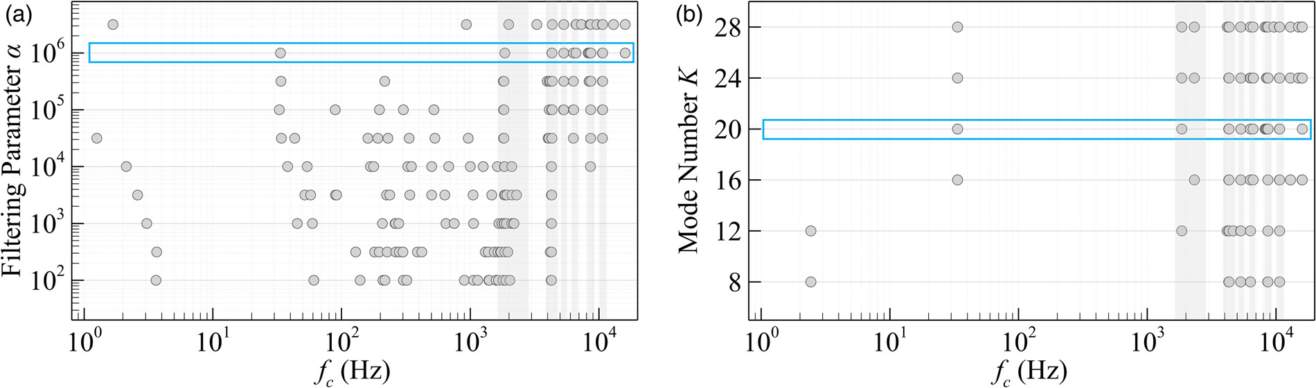
Figure 9 presents a comparison between the spatially averaged PSD of the reconstruction flow field using RVMD modes and time coefficients and the original space-time data. Within the frequency range of 0 to 20 kHz, the PSD peaks of the reconstruction data correspond well with those of the original data, validating the effective identification capability of RVMD for the main characteristics of the complete stall process. However, it should be noted that the RVMD technique is not perfect. In the region outlined by the blue dotted lines in Figure 9, there is a peak in the original data that disappears after RVMD reconstruction, indicating that RVMD failed to effectively identify the characteristics of this frequency band. The reasons for the aforementioned issues may lie in the fact that this paper did not employ the optimal filter parameter α and the number of modes K. In this paper, parameters are selected based on the identification effect of the PSD characteristic frequency bands, which can effectively identify overall characteristics but may not yield the most optimal decomposition results. In fact, distinguishing between different flow structures remains challenging, and defining “optimal decomposition” is still an unresolved issue. The parameter selection method used in this paper is not best but reliable based on the results. The characteristic frequency band not identified in Figure 9 exceeds 10 kHz, which is not significant in the stall process. Therefore, for the research objects in this paper, the issues of under-decomposition and over-decomposition present in RVMD do not affect the analysis of stall process.

Figure 9.

Comparison of spatially averaged PSD between original and reconstruction data.

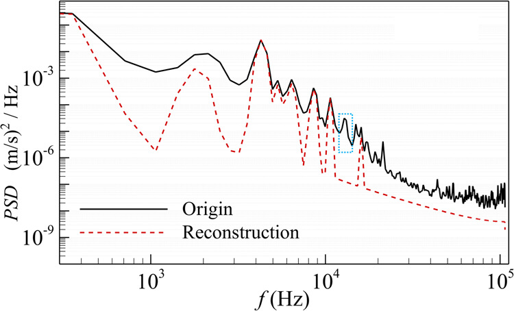
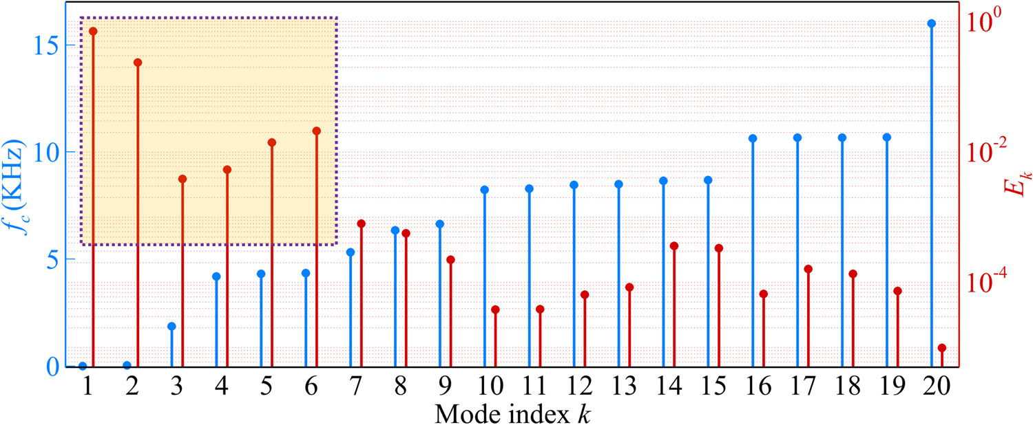
Figure 10 illustrates the relationship between the energy fraction of each mode and their central frequencies. For the complete stall process of the original CRAC, the energy is primarily concentrated in the first six modes, with mode1 and mode2 accounting for approximately 95.3% of the total energy. These two modes have very low frequencies, nearly approaching 0 Hz. Mode3 has a central frequency of 1,857 Hz, while modes 4 to 6 have central frequencies closely concentrated between 4,200 and 4,300 Hz. A series of modes in a flow field with frequencies that are close to each other should exhibit similar structures, because they are likely to represent the same true characteristic. However, the RVMD technique's over-decomposition may break a single structure into several modes. Subsequent analyses will focus on their primary modes. Figures 11 and 12 present the main RVMD mode contour maps and time evolution coefficients. In the figures, (a) to (f) represent mode1 to mode6, with the horizontal axis in the time coefficient representing the rotation periods. In the mode contour maps, E/ΣE is the ratio of a mode's energy to the total energy, while E/ΣE^∼ is the ratio excluding stable modes. Specifically, ΣE^∼ = ΣE-E₁-E₂. The time-evolution coefficient indicate the central frequency f_c of each mode.

Figure 10.

Relative energy and center frequency of RVMD modes.

Figure 11.

Contour map of RVMD modes of the CRAC.

Figure 12.

Time-evolution coefficients of RVMD modes of the CRAC.

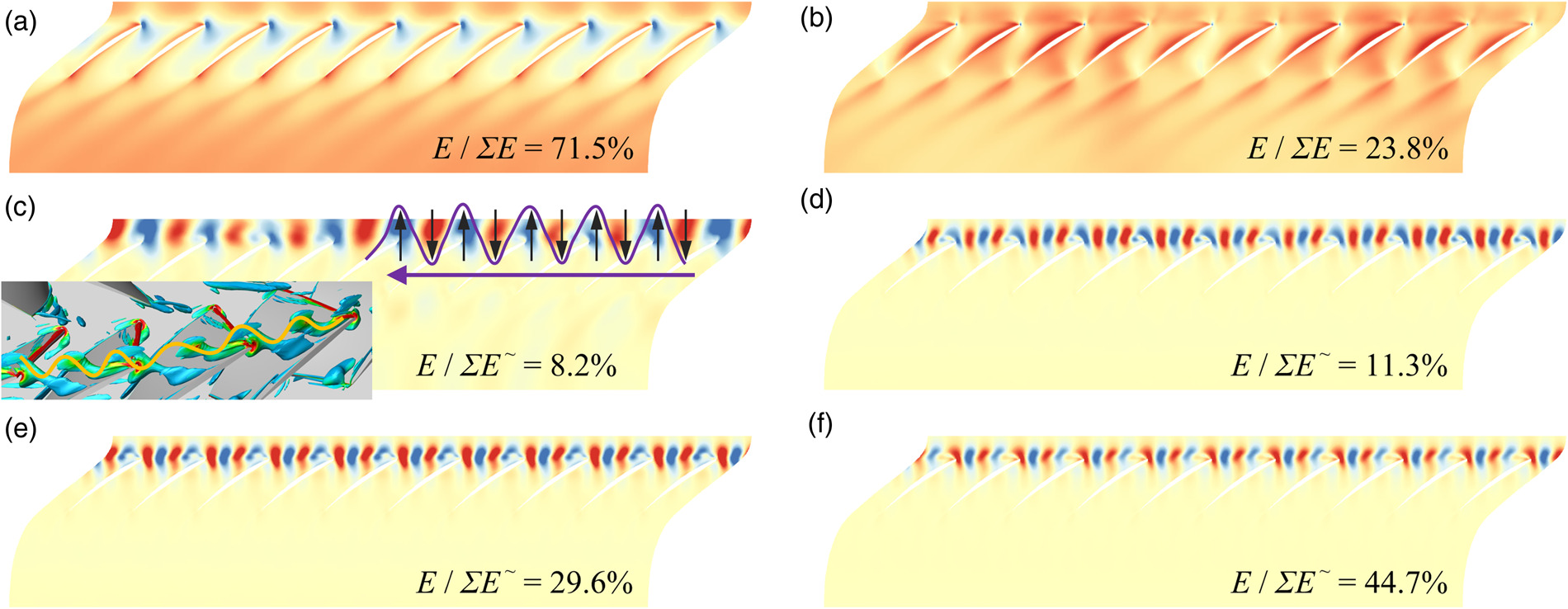
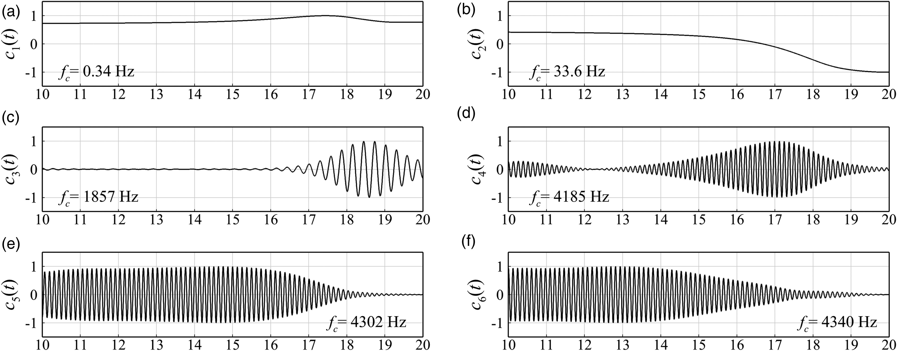
In Figures 11 and 12, mode1 and mode2 together characterize the evolution of the space-averaged value of V_z at the blade tip during the stall process. The contour maps of mode4 to mode6 (Figure 11d–f) are nearly identical, with strong fluctuation regions almost entirely overlapping the TLF coverage area. Moreover, these contour maps closely resemble the morphology of TLF, with central frequencies near 0.8 BPF. This frequency is nearly consistent with that of TLF structures found by Guo et al. (2023) using the DMD method on pressure fields. Thus, this paper concludes that mode4 to mode6 represent TLF structures throughout the stall process. The results indicate that TLF development during the stall process follows a characteristic pattern: initial strengthening, followed by weakening, and eventual dissipation, consistent with previous vortex structure evolution analysis.

The amplitude of the time coefficient for mode3 (Figure 12c) is essentially zero from T = 10 to T = 16, then rapidly increases and decays between T = 16 and T = 20. This evolution closely resembles the intermediate vortex shedding time coefficient reported by Liao et al. (2023), obtained using RVMD on the transient cylinder wake. Therefore, mode3 is considered to be a characteristic of the transitional state during the stall process. The contour map for mode3 (Figure 12c) shows an axially oscillating and circumferentially propagating flow structure, similar to that formed by the leading edge spillage of the R2 blade tip and TSVs shedding, as shown in Figure 6c. In other words, mode3 consists of two TSVs within the blade passage, creating positive and negative fluctuations. Between T = 16 and T = 17, the time coefficient of mode2 exhibits a rapid decline, indicating a reduction in flow through the blade tip passage and an increase in blockage. The rising adverse pressure gradient causes TSVs to move upstream, forming the mode3 characterized structure. The intensification of this structure coincides with the dissipation of the tip leakage structure, indicating that TSVs gradually replace TLVs as stall develops. As the degree of stall further intensifies, TSVs rapidly decay and dissipate under the influence of the backflow and the stall cells.

Integrating the earlier analysis of vortex structure evolution, here is a summary of the stall inception and development in the original CRAC. The TSV is the most critical structure in the inception and development of CRAC stall. Stall inception is marked by spillage from TSV collisions with adjacent blades on the R2 blade. During the stall inception, the tip flow velocity decreases and the adverse pressure gradient increases, causing the two TSVs to move upstream. One TSV interacts with the leading edge of an adjacent blade, causing spillage, while the other experiences vortex shedding between the leading edges. Both the LE spillage and the shed vortex are located on the inlet plane of the blade leading edge, and together form an axial fluctuation structure. This axial fluctuation structure slowly propagates circumferentially, periodically interacting with adjacent blades, accumulating and intensifying fluctuation energy, which disrupts and dissipates the TLV structure. In this process, the suppressive effect of the TLV on the TSV weakens, so the TSV intensity increases and the LE spillage further intensifies. Ultimately, the blade tip passage is completely blocked, backflow occurs at the TE, leading to a deep stall of R2.