
Introduction
Reynolds-averaged Navier-Stokes (RANS) simulations are the standard for complex flow simulations in industry, because the higher fidelity direct numerical simulations (DNS) and large eddy simulations (LES) are computationally too expensive for most applications. The RANS averaging introduces a term in the momentum equations that requires further modeling assumptions or simplifications, i.e. it is unclosed. This term is referred to as the Reynolds stress tensor and, over the past several decades, a large body of research has been devoted to its representation, namely the introduction of a turbulence model. Linear eddy viscosity models are a popular group of turbulence models that relate the strain rate tensor to the Reynolds stress anisotropy tensor through an isotropic eddy viscosity. Yet, because of their inherent assumptions they do not perform well on many realistic flows (Craft et al., 1996; Schobeiri and Abdelfattah, 2013). Particularly flows involving strong rotation or adverse pressure gradients, as encountered often in turbomachinery applications, represent a great challenge to turbulence models. It is indispensable for meaningful RANS predictions to have an estimate of the uncertainty in the simulations associated with the turbulence model. This type of uncertainty is directly related to the assumptions made in the model formulation, and therefore referred to as model-form uncertainty.
Data from experiments or from higher fidelity simulations presents an opportunity to enhance the predictive capabilities of RANS simulations. Traditionally, data has been used in the context of turbulence modeling only for model calibration and to define model corrections. Almost all turbulence models involve some empirical constants which are tuned to optimize the RANS predictions with respect to specific calibration cases. These calibration cases often are canonical flows such as decaying grid turbulence or plane homogeneous shear flow (Hanjalić and Launder, 1972). The quality of the resulting predictions depends on how relevant the calibration cases are to the case of interest. To extend the applicability of a turbulence models, corrections and modifications can be introduced, which also are calibrated on suitable data (Pope, 1978; Sarkar, 1992). Over the last decade, the main advancements of turbulence models, however, were made by capturing more physics, not by expanding the usage of data.
Recently, with the increased popularity of data science tools, efforts have been devoted to train machine learning models for RANS simulations. Some have incorporated sparse data into their simulations to improve predictions. There also have been efforts to use data to predict the Reynolds stresses, or to correct Reynolds stress predictions, as well as to identify and quantify uncertainty associated with the Reynolds stress predictions. Singh et al. (2017) used inverse modeling and trained neural networks to estimate a correction factor to the production term in the eddy viscosity transport equation of the Spalart-Allmaras turbulence model. They did not do formally quantify the uncertainty, but they studied the sensitivity of their predictions with respect to the training data set. Wang and Dow (2010) studied the structural uncertainties of the
In the present work, we are seeking an efficient data driven approach to quantifying uncertainty for general RANS models. As mentioned earlier, prior works in the literature either do not provide uncertainty estimates, they do so for specific models only, or they rely on expensive Monte Carlo sampling to characterize the uncertainty.
We are therefore introducing a data-driven framework based on an extension of the eigenvalue perturbations to the Reynolds stress anisotropy tensor developed by Emory et al. (2013). In the original approach, namely the data-free variant, the eigenvalues are uniformly perturbed to limiting states corresponding to 1, 2, and 3 component turbulence, leading to three independent simulations, in addition to the (unperturbed) baseline. However, perturbing everywhere in the domain leads to overly conservative uncertainty estimates because the model is assumed to introduce potential errors everywhere. The new, data-driven framework is used to predict a local perturbation strength in every spatial location based on the local mean flow quantities. The predictions carried out using the machine learning perturbations demonstrate that the uncertainty estimates provide credible quantification of the true modeling errors, and are more effective than the original data-free uncertainty estimates. We also carry out careful sensitivity analysis to grid resolution and inflow perturbations to confirm that the turbulence closure is the main source of uncertainty in the present test cases.
Turbulent separated flows in a diffuser
In turbomachinery applications, diffusers are used to decelerate the flow and increase the static pressure of the fluid. They are positioned downstream of compressors and turbines to increase their total-to-static isentropic efficiency. The operating principle is simply a change in cross-sectional area, but space constraints and reduction of losses often lead to configurations that are prone to flow separation and sensitivity to distortions of the incoming flow stream. Predictions of the turbulent flow in a diffuser represents the challenge in this work.
Test case setup
The turbulent flow in planar asymmetric diffuser first described by Obi et al. (1993) is considered. Figure 1 shows the setup: A channel is expanded from inflow width H to outflow width

The inflow is fully turbulent at
RANS simulations were carried out in OpenFOAM using the
Mesh sensitivity
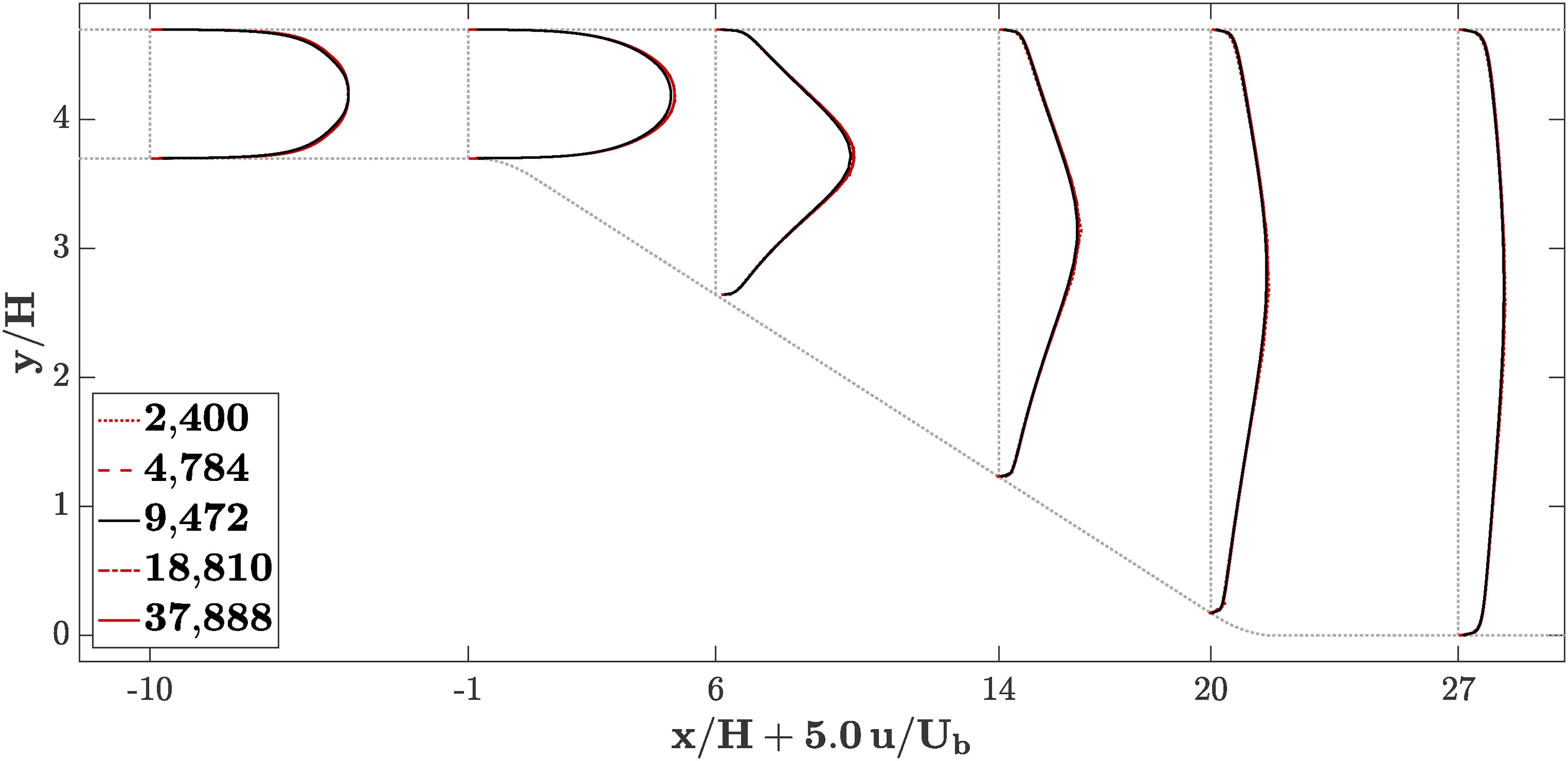
A mesh convergence study was performed using five levels: the baseline mesh and each two coarser and two finder meshes. The individual grid resolutions are given in Table 1, and the non-dimensional grid spacing of the wall-adjacent cells in the inflow section is
Inflow sensitivity
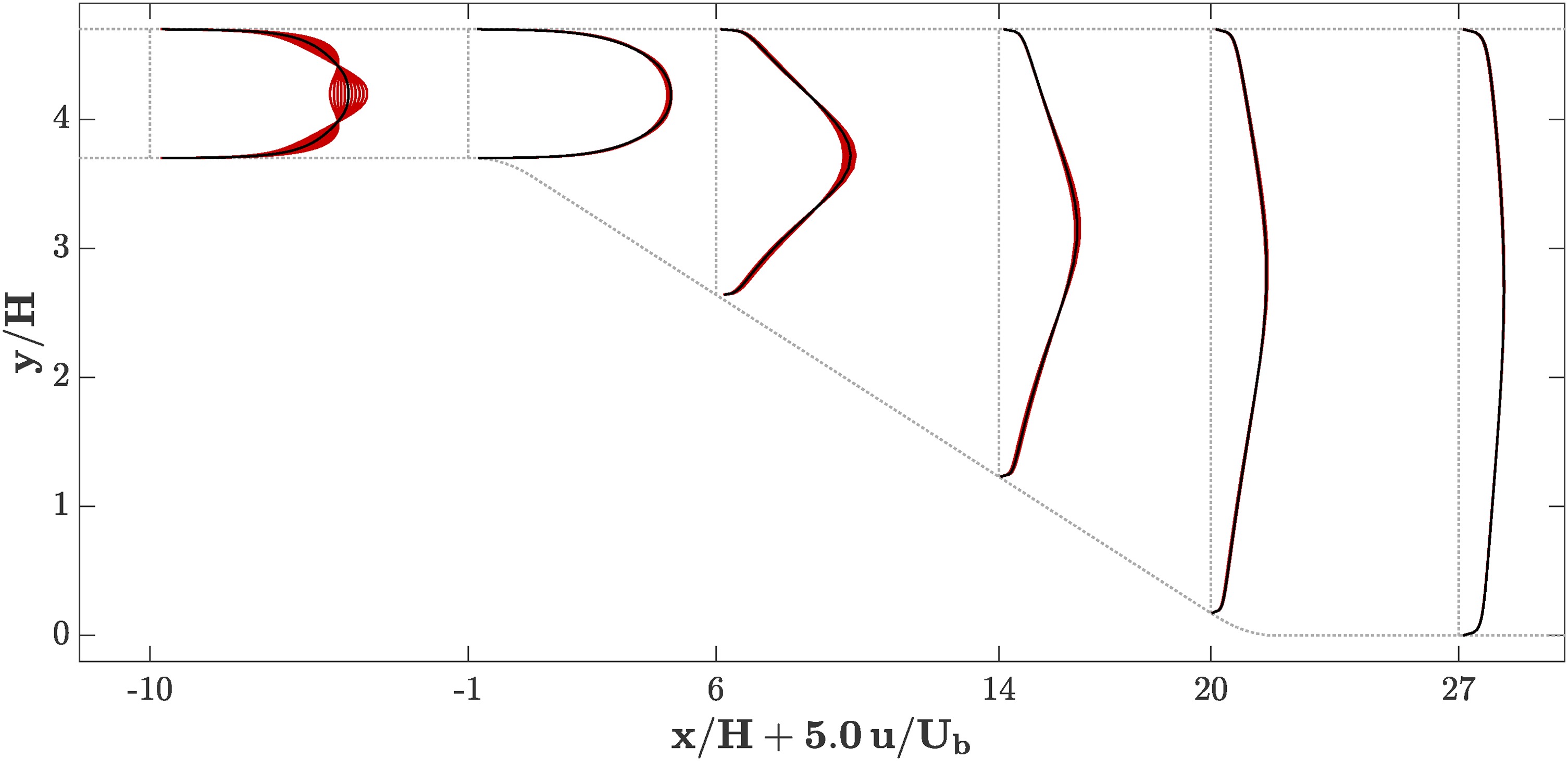
In order to build confidence in the predictions, the sensitivity of the solution to the inflow conditions was investigated. More specifically, the inlet velocity profile was distorted to vary the centerline velocity between
Validation
None of the simulations carried out so far indicate flow separation. Both the grid convergence and the inflow distortion studies provide confidence in the computations as very limited sensitivity to boundary conditions and numerical errors is observed.
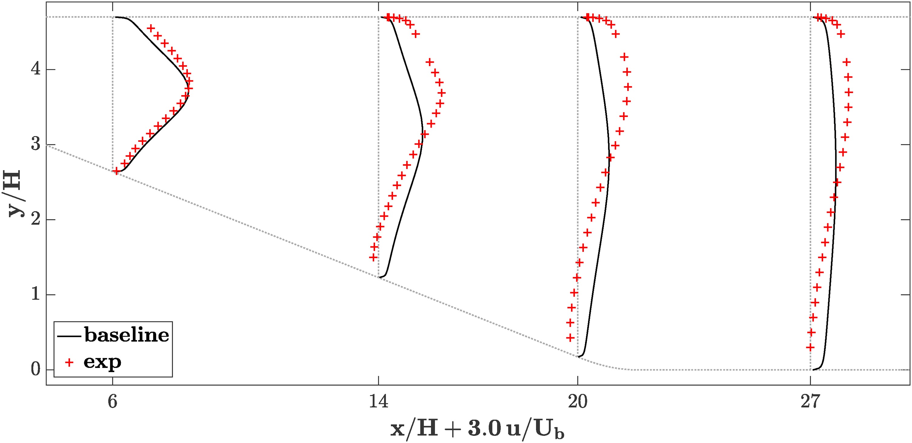
The baseline simulation is compared against experimental data from Buice and Eaton (2000) in Figure 4. While the flow remains attached at all times in the RANS simulation, the experimental data reveals the existence of a large flow separation that has not been captured by the simulation. The simulations are overpredicting the streamwise velocity in the lower half of the channel and underpredicting it in the upper half.
Data-free uncertainty quantification
The results presented so far illustrate a typical situation in computational engineering: simulations do not accurately represent experimental findings. Given the simplicity of the present application and the careful sensitivity analysis carried out to assess both numerical errors and boundary conditions, it is clear that the only source of inaccuracy in the simulations is the turbulence model. There is no shortage of different turbulence models (Iaccarino, 2001; Cokljat et al., 2003) that are known to provide better representation of the effect of adverse pressure gradients. However, it is useful to establish if it is possible to assess the effect of model inaccuracy and to estimate bounds on the predictions to understand the sensitivity of the results to the modeling assumptions.
Framework
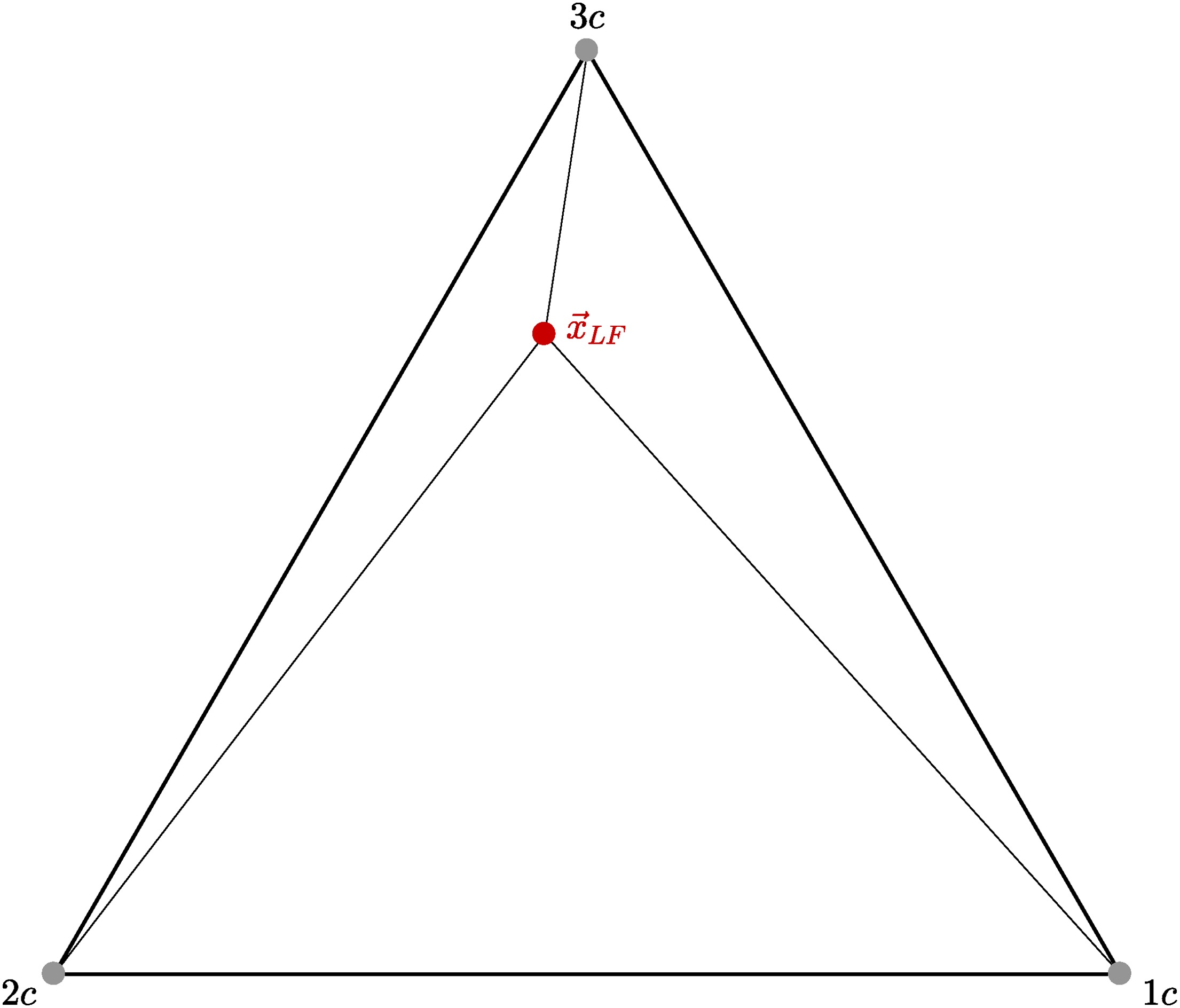
Emory et al. introduced perturbations to eigenvalues of the normalized Reynolds stress anisotropy tensor towards limiting states within the range of realizability (Emory et al., 2001, 2013). This technique is data-free and, in its basic form, parameter-free, and it allows to estimate model form uncertainty stemming from turbulence models. The starting point is to define the Reynolds stress anisotropy tensor
where
Figure 5.
Diffuser simulation. Profiles of streamwise velocity at different x locations with experimental data.
These eigenvalue perturbations add three perturbed simulations to the baseline calculations\comma \; one for each limiting state, leading to a total of four calculations. The uncertainty estimates are constructed by computing the range of values across the four calculations. The minimum and maximum values of the range form envelopes for any quantity of interest.
Validation
The framework of eigenvalue perturbations is applied to the present case of the planar asymmetric diffuser. Figure 6 shows the results of the baseline case, the uncertainty envelopes, and the experimental results. The uncertainty envelopes are constructed using the data-free eigenvalue perturbations towards each of the three limiting states with
The uncertainty envelopes cover the experimental results in most locations, and in particular at the bottom wall, where the perturbations suggest that the baseline calculation might be overpredicting the streamwise velocity. Unlike the mesh study and the inflow sensitivity study from the previous section, this analysis correctly indicates that there might be a region of flow recirculation at the bottom wall.
The uncertainty estimates, however, go beyond the experimental data, in some regions substantially, in other words seem to overestimate the modeling errors in some locations. This is expected because the perturbations are targeting all possible extreme states of turbulence anisotropy without consideration of their plausibility.
For practical applications, it would be useful to bound the uncertainty estimates more tightly, in order to have a more clear indication of the plausible modeling errors. The data-free framework perturbs the Reynolds stresses everywhere in the domain all the way to the respective limiting state. Yet, the Reynolds stress predictions of the turbulence model do not have the same level of inaccuracy throughout the domain. Therefore, it would be desirable to be able to vary the perturbation strength of the eigenvalue perturbations locally. That might allow to reduce the perturbation strength in regions, where less inaccuracy of the turbulence model is expected.
Data-driven uncertainty quantification
Perturbation strength
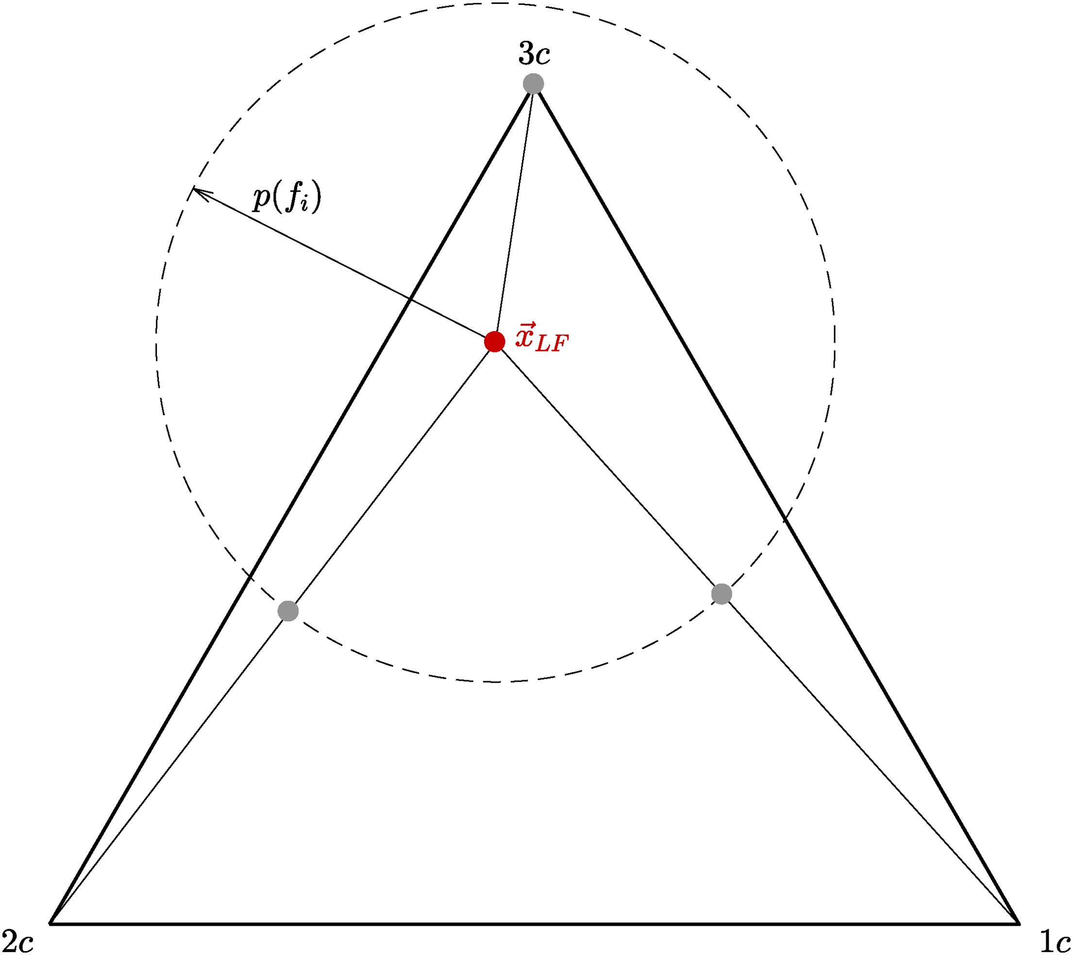
We study a data-driven approach to predict a local eigenvalue perturbation strength based on flow features. Here, we define the local perturbation strength
Machine learning model
A random regression forest is chosen as the machine learning regression model. Random forests are ensemble learners that are based on number of decision trees (Breiman, 2001). The details of regression trees and random forests are discussed in the following subsections. The random forest is implemented using the OpenCV library. More details on the implementation are provided in the appendix.
Regression trees
Regression trees are decision trees that are used to predict ordered variables (Breiman et al., 1984). Decision trees are algorithms that work by defining a hierarchical structure of nodes at which splits are performed. Starting from the root node, at each split one feature is compared against a corresponding threshold value. Depending on the difference between the feature values and the corresponding threshold, the algorithm continues at one of two child nodes. This continues until a so-called leaf node is reached, which assigns a value. Decision trees can be visualized in a tree like structure, hence the name, with the initial root node at the top and the leaves at the bottom.
They are built starting from the root and advancing recursively, finding the optimal split at each node. For the regression problem, the optimal split of a decision tree is the one that minimizes the root mean squared error over all features. Each regression tree is trained on a different random subset of the training set. Furthermore, at each node the optimal split is found for a random subset of features, called the active variables. Adding this randomness ensures that the individual regression trees are decorrelated. The value at a leaf node is the average over all the training samples that fall into that particular leaf node.
This structure enables regression trees to learn non-linear functions. They are also robust to extrapolation, since they cannot produce predictions outside the range of the training data labels, and to uninformative features, which are features that are considered but not relevant for problem (Ling and Templeton, 2015; Milani et al., 2017).
Random forests
Random forests are a supervised learning algorithm. They are ensemble learners, meaning that they leverage a number of simpler models to make a prediction. In this case of a random forest, the simpler models are regression trees.
In machine learning models, the means squared error can be decomposed into the squared bias of the estimate, the variance of the estimate, and the irreducible error:
where
In many machine learning models one can vary the model flexibility. A more flexible model is able to learn more complex relationships and will therefore reduce the bias of the predictions. At the same time, a more flexible model increases the likelihood of overfitting to the training data and thereby of increasing the variance. The search for the optimum model complexity to achieve both low bias and low variance is commonly referred to as the bias-variance trade-off.
Binary decision trees are very flexible and tend to overfit strongly to the training data. Hence, they have a low bias and a high variance. Random forests base their predictions on a number of decorrelated decision trees. Decorrelation is achieved by bagging, which is the training on random subsets of the training data, as well as randomly sampling the active variables at each split. Since the trees are decorrelated, the variance of the random forest predictions is reduced and generalization improved. At the same time, random forests are able to keep the low bias of the decision trees. This makes random forests, despite their simplicity, powerful predictors for a range of applications (Breiman, 2001).
Features
Decision trees, and machine learning algorithms in general, require the definition of a set of features that represent the mapping from input to outputs.
In the present scenario, i.e. an incompressible turbulent flow, a set of twelve features was chosen. In order to be able to generalize to cases other than the training data set, all features are non-dimensional. The computation of the features requires knowledge of the following variables, which are either constant or solved for during the RANS calculations: the mean velocity and its gradient, the turbulent kinetic energy as well as its production and its dissipation rates, the minimum wall distance, the molecular viscosity, and the speed of sound.
The list of features is given in Table 2. For vectors the L2 norm, and for second-order tensors the Frobenius norm is used. The first five features are traces of different combinations of the mean rate of strain and mean rate of rotation tensors, normalized by the turbulence time scale. One other normalization was tested, using the mean strain and mean rotation time scales, yet using the turbulence time scale yielded better results, i.e. smaller overall MSE. The sixth feature is a non-dimensionalized Q criterion, which is commonly used to define vortex regions. The seventh feature is the ratio of the turbulence kinetic energy production rate to its dissipation rate, governing the turbulence kinetic energy as a key parameter in characterizing the turbulence of the flow. Next are the ratio of turbulence to mean strain time scale, the Mach number, and the turbulence intensity. The turbulence Reynolds number, which can also be interpreted as a non-dimensional wall distance, is the eleventh feature. Finally, a marker function indicating deviation from parallel shear flow is used as a feature, as scalar turbulence viscosity models are geared often geared towards and validated on such parallel shear flows (Gorlé et al., 2012).
Table 2.
Non-dimensional features used for the random regression forest.
The following variables are used: the mean rate of strain and its norm
Training case setup
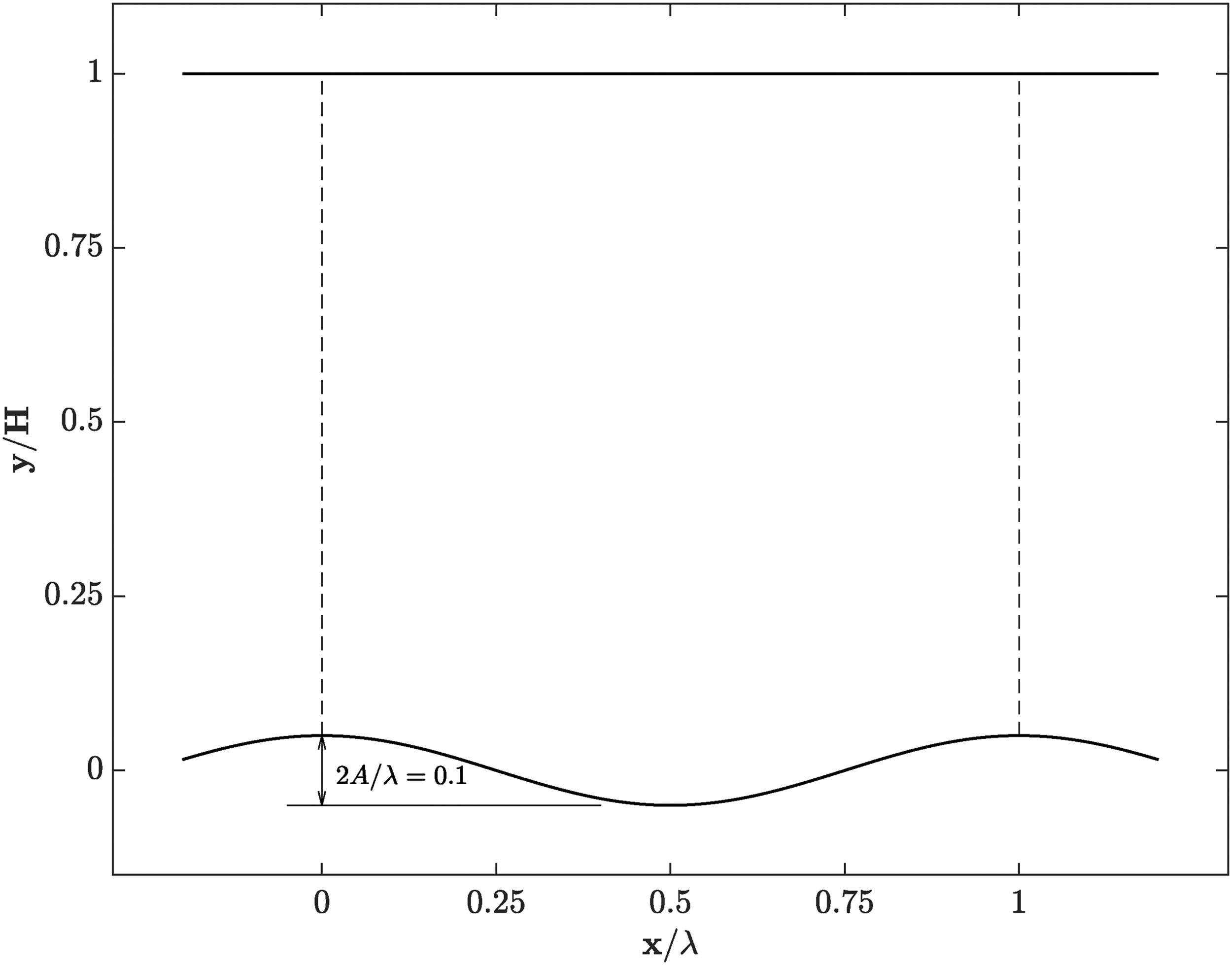
Training data is used to determine the model parameters, not to evaluate the model’s performance, because unlike the test case it cannot provide an unbiased model assessment. The periodic wavy wall case was used to obtain training data for the random regression forest model. It is defined as a turbulent channel with a flat top wall and a sinusoidal bottom wall as illustrated in Figure 8. The ratio of channel height to wave length is
Training case mesh sensitivity
The simulations use a structured grid with a resolution of 16,384 cells, 128 in each the x and the y direction. The computational domain covers the space from one wave crest to the next one as indicated by the dashed lines in the figure, with periodic inflow and outflow boundary conditions. A mesh convergence study was carried out with two coarser and two finer meshes. The factor between the total number of cells is approximately 2 between the refinement levels, and the individual grid resolutions are given in Table 3. Figure 9 is showing profiles of the streamwise velocity for the mesh convergence study. There is barely any difference between the different calculations. Features for the random forest training were computed from the baseline case, and labels were computed from both the baseline case and higher fidelity data, with each RANS grid node being one data point. The labels are defined as the actual distances in the barycentric domain between the location predicted by the baseline calculation and the higher fidelity one. The higher fidelity data is statistically converged DNS data from Rossi (2006), which was linearly interpolated to the RANS cell locations using the nearest four DNS cell locations for each RANS cell.

Hyperparameters
In machine learning models, hyperparameters are parameters that are not learned during model training, but that instead are set before training and used to define the functional form of the model and control the learning process. The impact of four different hyperparameters on the learning of the random regression forest model is studied: the maximum tree depth, the minimum sample count, the active variable count, and the number of trees. The minimum sample count is the minimum number of samples required at a particular node in order to do further splitting. The active variable count is the number of features randomly chosen at each node to find the optimal split. For each of the first three hyperparameters a couple of different values were studied over a range of 1 to 200 regression trees. Figure 10a–c show the training and testing error of the random forest training of those studies plotted against the number of trees. Each solid line corresponds to the training error for a specific value of the particular hyperparameter, and each dotted line corresponds to the testing error. To improve readability, these errors are plotted for every third number of trees only. For these studies, the dataset was first randomly shuffled and then split into a training set comprising
Figure 10.
Training error (solid) and testing error (dotted) vs. number of trees for different (a) maximum tree depth values, (b) minimum sample count values, and (c) active variable count values.
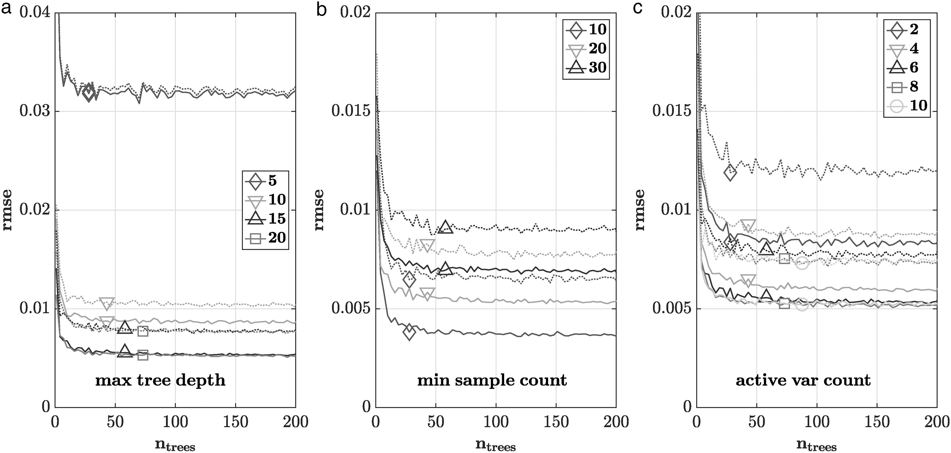
The results from the maximum tree depth study are shown in Figure 10a. The training and test errors are plotted in solid and dotted lines, respectively, against the number of trees. The tested values are 5, 10, 15, and 20. There is no significant difference between 15 and 20. The errors are a bit larger for 10 and significantly larger for 5, which clearly outperformed all other cases in terms of generalization. Because it showed the best performance for training and test error, a maximum tree depth of 15 was chosen. 20 was not chosen, because it increased computational costs without improving prediction performance.
Figure 10b shows the results from the minimum sample count study. The tested values are 10, 20, and 30. All three cases could do better in terms of generalization, with the cases with the larger minimum sample counts doing slightly better. In turn, the overall performance clearly is improving with smaller values. Because the enhanced performance for the smaller values was more clear than the reversed gain in generalisation, 10 was chosen as minimum sample count.
The number of active variables was varied between 2 and 10 at an increment of 2 as shown in Figure 10c. The results do not vary greatly in terms of generalization. Larger numbers of active variables lead to lower training and test errors. The training errors for 6, 8, and 10 are the lowest and do not differ significantly. The test error for 6 is slightly larger than for 8 and 10. 8 was chosen as active variable count, because shows overall a better performance than smaller values while leading to a stronger decorrelation between the individual regression trees than the similarly performing case with value 10.
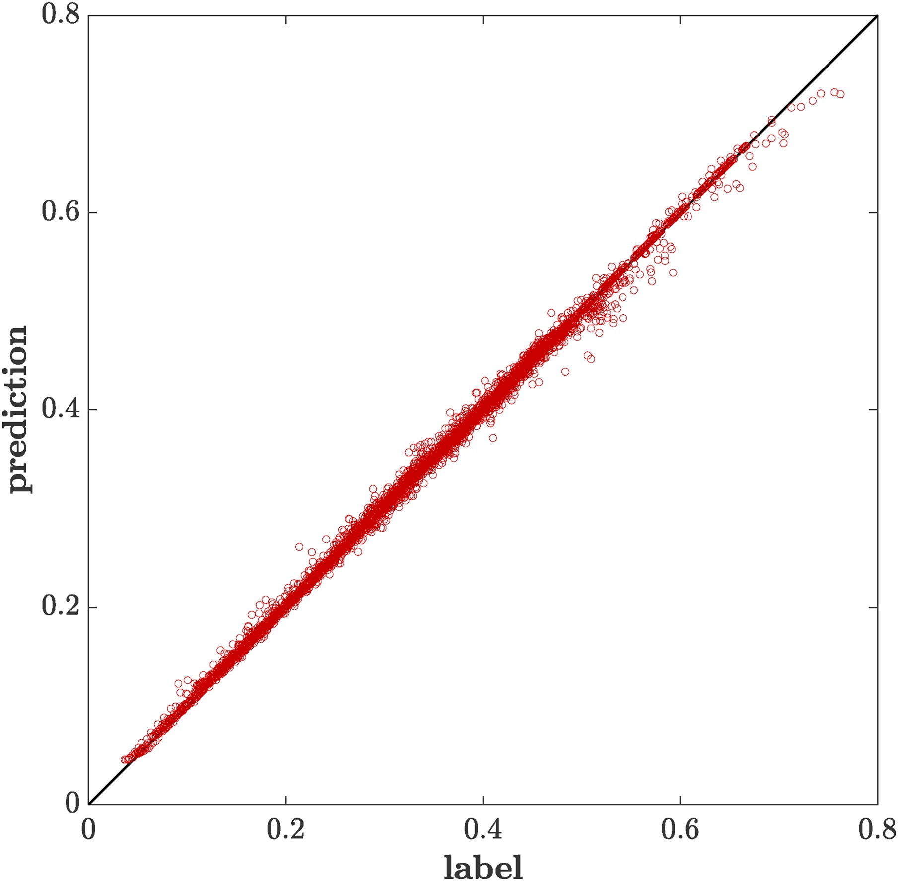
Over all three preceding hyperparameter studies the impact of the number of trees can be observed. There is a steep gain in performance for small numbers of trees followed by a quick saturation. The computational costs of evaluation a random forest model scale linearly with the number of trees. Therefore, the minimum number of trees for maximum model performance is sought. In none of the cases, significant improvement was observed for a number of trees exceeding 50. Therefore, the final random regression forest was trained for 50 regression trees on the whole dataset. The root mean squared error is
Feature importance
The OpenCV library used to train the random regression forest allows for the computation of feature importance, i.e. a quantitative assessment of the impact that each feature has on the final prediction. Table 4 presents the normalized feature importance scores. There is still a lot to learn about the importance of different features for data-driven uncertainty quantification, but we will make a few initial observations.
Table 4.
Normalized feature importance scores.
The two most important features of the trained model are the non-dimensional wall distance and the marker indicating deviation from parallel shear flow. The flow features in the present cases that are the most challenging for turbulence models are flow separation, flow reattachment, and development of a new boundary layer. All these features occur at or near the wall, supporting the significance of the wall distance. The marker for deviation from parallel shear flow was developed specifically to identify regions where the linear eddy viscosity assumption becomes invalid (Gorlé et al., 2014). The importance of this feature indicates that the model was able to highlight this relationship.
The features based on combinations of the mean rate of rotation were clearly more important than the ones based on combinations of the mean rate of strain, with the trace of the squared mean rotation rate tensor being ranked as third most important feature. Other relevant features are the Q criterion, identifying vortex regions, and the turbulence intensity. The turbulence level naturally has an impact on the accuracy of the turbulence model. As expected the divergence of the velocity is not a significant feature for this incompressible flow case.
It is important to point out that the feature importance is strongly related to the baseline turbulence model and related to the training dataset.
Validation
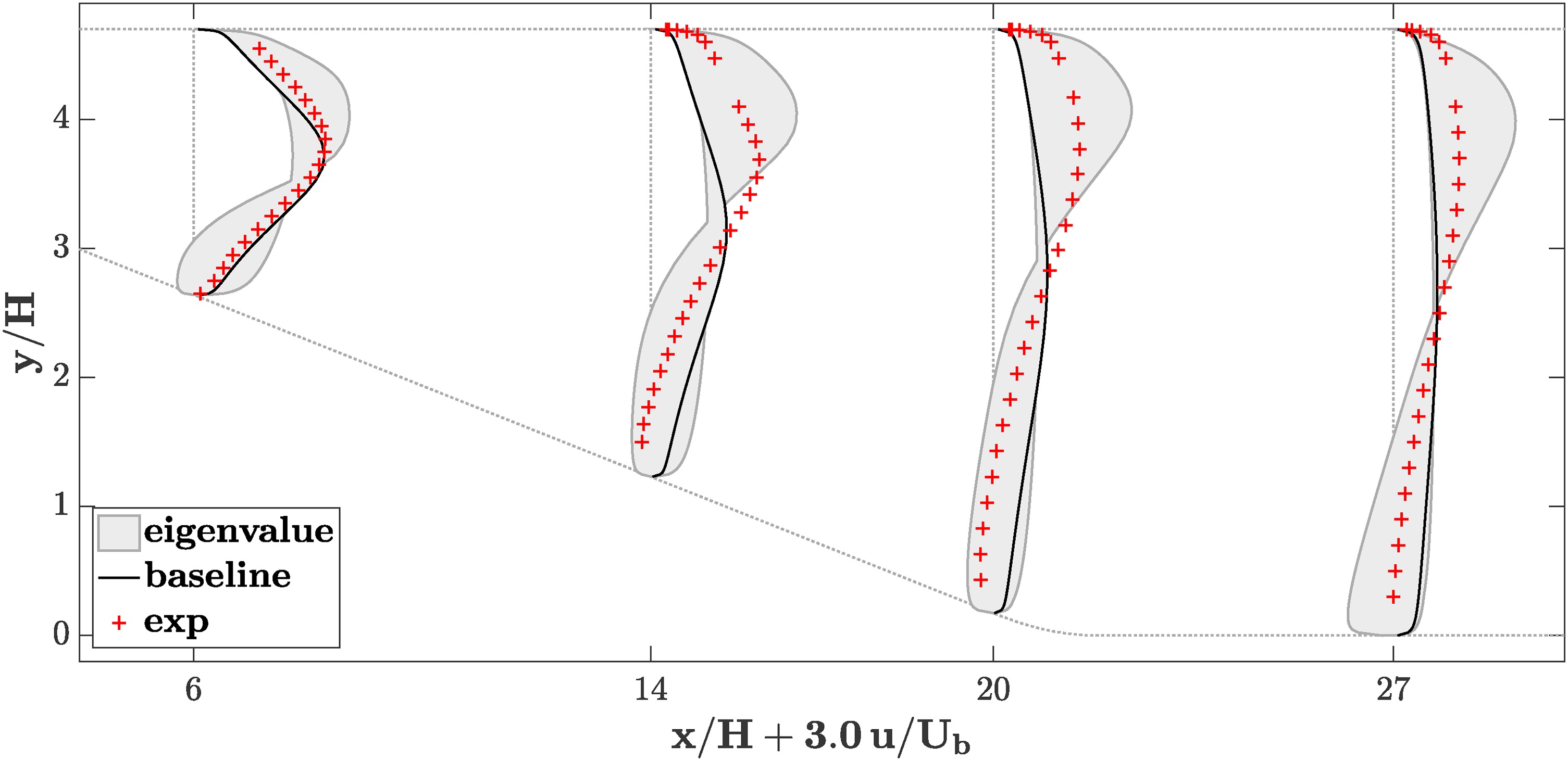
Finally, this new, data-driven framework was applied to the planar asymmetric diffuser. The random forest model was used to predict a local perturbation strength at every cell during the RANS calculations. As for the data-free uncertainty envelopes, three perturbed calculations were carried out for the three limiting states of turbulence. Figure 12 shows the results of the baseline case, the results of the uncertainty bands from the data-driven eigenvalue perturbations, and the experimental results.
Figure 12.
Data-driven, local eigenvalue perturbation. Profiles of streamwise velocity at different x locations.

The uncertainty envelopes still display the same general trend, suggesting an overprediction of the streamwise velocity in the lower half of the channel. As expected from permitting smaller perturbation strengths, the envelopes are narrower than they are when using the data-free framework from the previous section. There are no regions where the uncertainty is substantially overestimated: In most regions, the envelopes reach just up to or at least very near to the experimental data. Thus, for the test case the data-driven uncertainty estimates give a reasonable estimate of the modeling errors and therefore the true uncertainty in the flow predictions.
Conclusion and future work
This study is the first step into using data to enhance uncertainty estimation. Based on an existing data-free framework, a new, data-driven approach was introduced in which the perturbations to the Reynolds stress anisotropy eigenvalues is estimated using computable flow features. A random forest was trained on a wavy wall high-fidelity dataset and tested on the prediction of the turbulent separated flow in a diffuser case, with promising early results. The newly predicted uncertainty envelopes closely tracks the experimental data. At the same time, there are still a number of open questions and directions for future work on this topic.
For this study, only one training case and one test case were used. One open question is what impact the choice of the training case(s) has on the results of the test case(s) in this framework. The two cases were relatively similar in terms of the flow features they exhibit, and we expect that this is a necessary condition for accurate uncertainty predictions. Using training data from different cases could make the model applicable in a wider range of test cases.
Just like the choice of test case, the choice of features is an aspect that requires further investigation. This process could be informative for learning which flow features have a stronger impact on uncertainty in the flow predictions. Similarly, the non-dimensionalization of the features gives room for exploration, which again is crucial for generalization. A different time scale was tested for some of the features, but there are more options to consider.
Lastly, different choices could be made regarding the machine learning model. The current choice is a random regression forest. A hyperparameter study was used to decide on a set of parameters, but their effect on the results of the test case are not conclusive. To reduce computational expenses, it would be compelling to find the minimum number of trees needed before the quality of the uncertainty predictions breaks down. And beyond random regression forests, it is useful to compare different types of machine learning approaches.