
Introduction
NICFD is a new branch of fluid-mechanics 32 concerned with the flows of dense vapors, supercritical fluids, and two-phase fluids, in cases in which the ideal gas law does not apply.
In these flows, the isentropic variation of the speed of sound with density is different if compared to the flow of an ideal gas 12; thus, the flow field is bound to be quantitatively 21 or even qualitatively different 54.
NICFD internal flows occur in numerous heterogeneous industrial processes. The supersonic and transonic flow through an ORC turbine nozzle is an example 10. Another case in the energy sector is the transonic flow occurring in the compressor of supercritical CO2 power plant 35, or of CO2 capture and sequestration plants 3. Similarly, flows of fluids in dense-vapor or two-phase conditions are relevant in throttling valves, compressors, and ejectors of refrigeration and heat pump systems 5, 4. Turbomachinery and nozzles partly operating in the NICFD regime are common in the oil and gas industry 7, 24, 33, and these unconventional flows can also occur in pipelines for fuel distribution 49. Dense vapors made of heavy molecules can be used in supersonic wind tunnels instead of air to achieve higher Reynolds numbers, which can be varied almost independently from the Mach number 2. Finally, supercritical CO2 nozzle flows are used in the pharmaceutical industry to extract chemicals 50.
The technical and economic viability of these processes can be greatly enhanced if the performance of fluid flow components is improved. Fluid-dynamic shape optimization (FSO) arguably allows a quantum step progress in this respect 30. FSO has played a crucial role in the development of more conventional technologies 23, 25, 38, but it can be even more important in the case of technologies entailing NICFD flows, where design experience and experimental information are much more limited. Hence, concerted research efforts have been recently devoted to develop FSO techniques for NICFD applications, in particular for nozzles and turbomachinery blades 22, 39, 40, 16, 36.
The FSO of nozzles and of turbomachinery blades can be performed with either gradient-free 27 or gradient-based 28 methods. Gradient-free algorithms only demand the evaluation of the objective function (e.g., genetic algorithms), and they are often coupled with surrogate models to reduce the computational cost 38, 45. Nevertheless, the number of function evaluations necessary to converge to an optimum solution are comparatively large, and only few design variables can be concurrently optimized 41. Instead, gradient-based methods can reach an optimal solution in far fewer iterations. However, these techniques require not only the computation of the objective function, but also the expensive estimation of its gradient with respect to the design variables. The use of the adjoint method makes the computational cost of the gradient evaluation of the same order of magnitude of that of the objective function, regardless of the number of design variables 37. Thus, if the problem involves a large number of design variables and the estimation of the objective function is computationally expensive, adjoint-based methods are the only viable technique.
The already difficult task of linearizing the flow equations 52 becomes even more challenging in the context of NICFD, where complex thermo-physical fluid models must be adopted to accurately estimate fluid properties, raising the need of specialized numerical methods 9, 42. Despite that, recent work on the subject 39, 40 has demonstrated the potential of adjoint-based method for the FSO of NICFD flows occurring in ORC turbine cascades. However, this approach was limited to inviscid flows, restricting the adjoint applicability to some supersonic flow cases where viscous effects are negligible.
In this work the adjoint method was extended to fully-turbulent NICFD flows; thus, the approach can be applied, without restrictions, to the FSO of any NICFD application. The adjoint solver was obtained by linearizing the discretized flow equations by means of AD. Nevertheless, the use of AD, if performed by differentiating individual subroutines like in 39, still requires additional error-prone steps whenever new numerical schemes or fluid models are added to the source-code. On the contrary, in this work a holistic linearization approach was adopted, whereby AD is applied in a black-box manner to the entire source code. This is accomplished with the help of modern meta-programming features 44 in combination with a reformulation of the state constraint into a fixedpoint problem 1. The result is a fast and accurate discrete adjoint solver that includes all the flow solver features, such as arbitrary complex equations of state and turbulence models.
The new Reynolds-averaged Navier–Stokes equations (RANS) adjoint solver was developed by leveraging on the open-source software infrastructure of SU2 15, a platform conceived for solving multi-physics PDE and PDE-constrained optimization problems using general unstructured meshes. The SU2 flow solver, previously extended to model NICFD flows 51, was adapted to simulate turbomachinery flows.
The developed adjoint solver was naturally integrated into the automatic constrained FSO framework already available in SU2. The optimizer uses the objective function and constraint sensitivities to accordingly re-shape the target geometry by moving the control points of a free-form deformation box. To avoid re-meshing at each design cycle, a linear-elasticity method is applied to propagate the surface perturbation to the entire mesh.
The capability of the new design tool was tested on two exemplary cases: a supersonic and a transonic ORC turbine cascade. The results demonstrate the importance of accurately modeling non-ideal thermodynamic and viscous effects for adjoint-based FSO applied to NICFD applications.
This article is organized as follows. The next section describes the SU2 flow solver and its extension to accurately simulate and analyze turbomachinery NICFD flows. The Fluid Dynamic Design Chain section focuses on the derivation of the discrete adjoint solver, also taking into account the surface and volume mesh deformation. The Results and Discussion section reports the application of the new adjoint solver to the re-designing of two typical ORC blades, and discusses the different results obtained using a turbulent or an inviscid approach. Finally, in the last section, before the conclusions, the more accurate NICFD approach is compared with the more standard ideal-gas based method.
Flow solver
Spatial and time discretization
The RANS equations are discretized in SU2 using a finite volume method with a standard edge-based structure on a dual grid with control volumes that are constructed using a median-dual vertex-based scheme 15. The PDE semi-discretized integral form is
where R(U) is the residual vector obtained by integrating the source term over the control volume Ω and summing up all the projected numerical convective and viscous fluxes associated with all the edges of Ω.
Ad-hoc methods must be used to compute numerical fluxes that are independent from the thermodynamic model of the fluid. For example, the Roe scheme 43 in the generalized formulation presented in 31 was implemented in SU2 51.
The time integration is performed with an implicit Euler scheme resulting in the following linear system:
where ∆Un := Un+1−Un and ∆tn is the (pseudo) time-step which may be made different in each cell by using the local time-stepping technique 34. (2) can be solved using different linear solvers implemented in the code framework 15. Furthermore, non-linear multi-grid acceleration 8 is available.
Non-reflecting boundary conditions
Non-reflecting boundary conditions (NRBC) were implemented according to the method proposed in 17. Any incoming boundary characteristic
The harmonic boundary solution
When NRBCs are imposed at the inlet boundary, the computed average entropy, stagnation enthalpy, and flow direction can differ from the user-specified values 18. Therefore, to ensure that a correct solution is found, the average incoming characteristics are computed by driving the difference between the computed average quantities and the user-specified quantities, i.e.,
to zero at each time step. The resulted non-linear system
is solved via a Newton-Raphson iteration, where the Jacobian of the residuals with respect to the characteristic variables for an arbitrary thermodynamic model can be written as
(6)
The expression of the enthalpy derivatives and the entropy derivatives are available in SI (i).
The same problem occurs at the outflow boundary; thus, the average incoming characteristic is determined in such a way the exit pressure at convergence is the same as that specified by the user. Since the pressure is directly related to the variation of the incoming characteristic, the average change on the fourth characteristic can be directly computed as
Equation (7) is also used in case of supersonic outflow conditions whereby the normal component of the outflow Mach number is subsonic.
Once the average and the harmonic component of each incoming characteristic, and the local outgoing characteristic have been computed, the characteristic change at the boundary nodes can be converted back into the change of the primitive variables. This change is summed to the equivalent average values, around which the flow equations are linearized at the boundary. The primitive variables are averaged using the mixed-out procedure, which is the only physically consistent method for averaging flow quantities 47. The updated values of the primitive variables are used to compute the boundary conservative variables, which, in turn, are used to calculate the convective and the viscous numerical fluxes for the residual in (1).
Fluid dynamic design chain
Dependence of the objective function from design variables
Figure 1 schematically shows the dependence of the objective function,
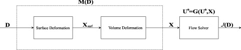
The use of the surface nodes as design variables (i.e., D = Xsurf) may lead to discontinuous solutions. Thus, the control points (CP) of a Free-Form Deformation (FFD) box were selected as a design variables 48. The surface variation imposed by a perturbation of the FFD CPs is propagated through the volume mesh using the linear elasticity theory as proposed of 14.
Discrete adjoint solver
The discrete adjoint solver was implemented following the approach in 1. Based on the design chain described in 3a, the optimization problem is formulated as
Following the fixed point iteration approach, the constraint on the solution, Equation (10), is the method to solve the flow equations itself described in Equation (2). M(D), instead, is a linear function that formally contains the surface and the volume mesh deformation as shown in Figure 1.
The Lagrangian associated to this problem is
where the shifted Lagrangian N is
and
Similarly to the iterative method used for the solution of the flow equations, Equation (10), the adjoint equation, Equation (15), is solved iteratively with the fixed-point iteration:
where U* is a numerical solution of the flow equations. Once the adjoint solution,
Gradients evaluation with algorithmic differentiation
Algorithmic Differentiation, also known as Automatic Differentiation, is a method to calculate the derivative of a programmed function by manipulating the source-code 20. As an example, consider a generic function y = f(x). It can be demonstrated that the product
where
The open-source AD tool CoDiPack 44, which had been already successfully applied to SU2 1, was also selected for this work. Compared to other AD approaches, CoDiPack exploits the Expression Templates feature of C++. This approach introduces only a small overhead in terms of statement run-time. Thus, the black-box application of AD to complicated non-linear iterative functions becomes feasible. Furthermore, this method is computationally efficient whenever there are code parts containing statements that are not directly involved in the calculation of derivatives, which avoids to perform the extensive derivative-dependency analysis that is necessary in most applications of AD 6.
Results and discussion
The capabilities of the FSO method described in Section 3 were demonstrated by redesigning a supersonic and a transonic cascade that are representative of typical cascades adopted in single-stage and multi-stage ORC turbines 11. The illustration of the two test cases follows the same structure. First, the gradient validation is reported, in which the adjoint sensitivities of the objective function and constraint were compared with their finite-difference (FD) equivalent. Second, the results of the optimization are documented. Lastly, the optimization results obtained with the inviscid flow and adjoint solver are also discussed and compared with the ones obtained with the RANS solvers.
In both test-cases the chosen working medium was the siloxane MDM, modeled with the polytropic Peng-Robinson (PR) EoS. The parameters of the model are listed in Table 1. A detailed description of the implementation of the PR EoS in SU2 is available in 51. Turbulent computations were carried out with the k-ω SST model 29, ensuring wall y+ below unity along the blade surface. The optimizer is the minimize routine of the python library scipy.optimize. This routine implements the Sequential Least SQuares Programming (SLSQP) algorithm introduced in 26.
Table 1.
Peng-Robinson EoS parameters for the MDM organic fluid.
| Fluid | MDM | - |
| R* | 35.23 | [Jkg−1K−1] |
| γ | 1.02 | [-] |
| Tcr | 564.1 | [K] |
| pcr | 1.415 | [MPa] |
| θ | 0.529 | [-] |
Supersonic cascade
The supersonic cascade considered in this work was previously investigated and documented in 10, 39, 40. The simulation of the flow around the baseline geometry shows that significant fluid-dynamic penalties would be present because of a strong shock-wave forming on the rear suction side of the blade. Therefore, to improve the cascade performance, the entropy-generation rate,
The boundary conditions for the simulation are summarized in Table 1. Although total inlet temperature and pressure quantities were given as input for the inflow conditions, these are internally converted to total enthalpy and entropy, which are eventually imposed at the boundary (cf. Equation [4]).
Table 1.
Inlet and outlet boundary conditions values for the supersonic cascade test-case.
| Ttot,in | 545.1 | [K] |
| ptot,in | 0.80 | [MPa] |
| βin | 0.0 | [°] |
| pout | 0.10 | [MPa] |
| Itur,in | 0.03 | [-] |
| 100.0 | [-] |
According to the convergence study on the baseline geometry, a maximum number of 1,200 iterations was set for both the flow and the adjoint solver, and the solutions were obtained with an implicit time-marching Euler scheme with a CFL number of 40 on 44,000 grid points mesh.
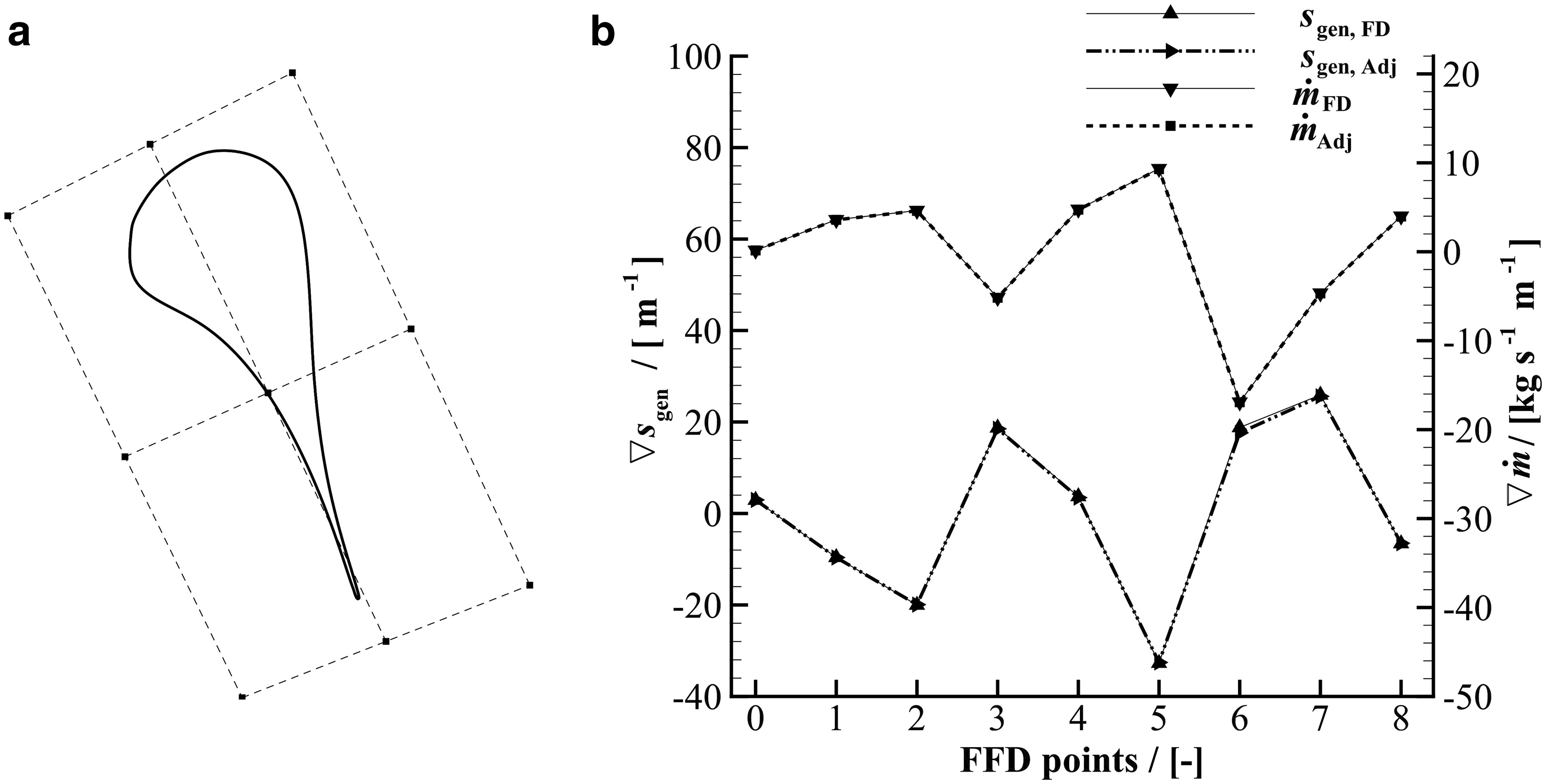
The gradient of the objective function and constraint were first validated against FD. To ease the process, a simple FFD box of 9 CPs was selected (Figure 2), and the validation was conducted by using a FFD step-size equal to 1E-05. Figure 2 shows that the objective function and constraint gradient provided by the NICFD adjoint very accurately correlate with the correspondent FD values. This result is also a confirmation that the selected convergence criterion guarantees an accurate estimation of the gradient.
Figure 2.
Objective function and constraint gradient validation for the supersonic cascade test-case.
a) 2D FFD box of degree two on both directions (9 CPs) used for the validation; b) comparison between the FD and adjoint gradient values.
Differently from the validation, in which the process can be considered FFD-degree independent, the FFD box for the optimization is composed by 121 CPs, as can be seen in Figure 3. This choice was made to ensure a high level of design flexibility, which is of primary concern for cascades operating in the supersonic regime, for which slight geometrical modifications can lead to largely different performance. In addition, to prevent unfeasible designs, the sensitivity around the trailing-edge was nullified at each optimization iteration. This has a twofold effect. First, it ensures that a minimum acceptable value of the blade thickness is maintained, without directly introducing a geometrical constraint on the thickness distribution. Second, it alleviates mesh deformation issues at the trailing-edge. To guarantee a smooth convergence, the step size of the SLSPQ optimizer was under-relaxed with a value equal to 1E-05 for both the objective function sensitivity and the constraint sensitivity.
Figure 3.
Supersonic cascade optimization.
a) 2D FFD box of degree 10 on both directions (121 CPs) used for the optimization; b) optimization convergence history.
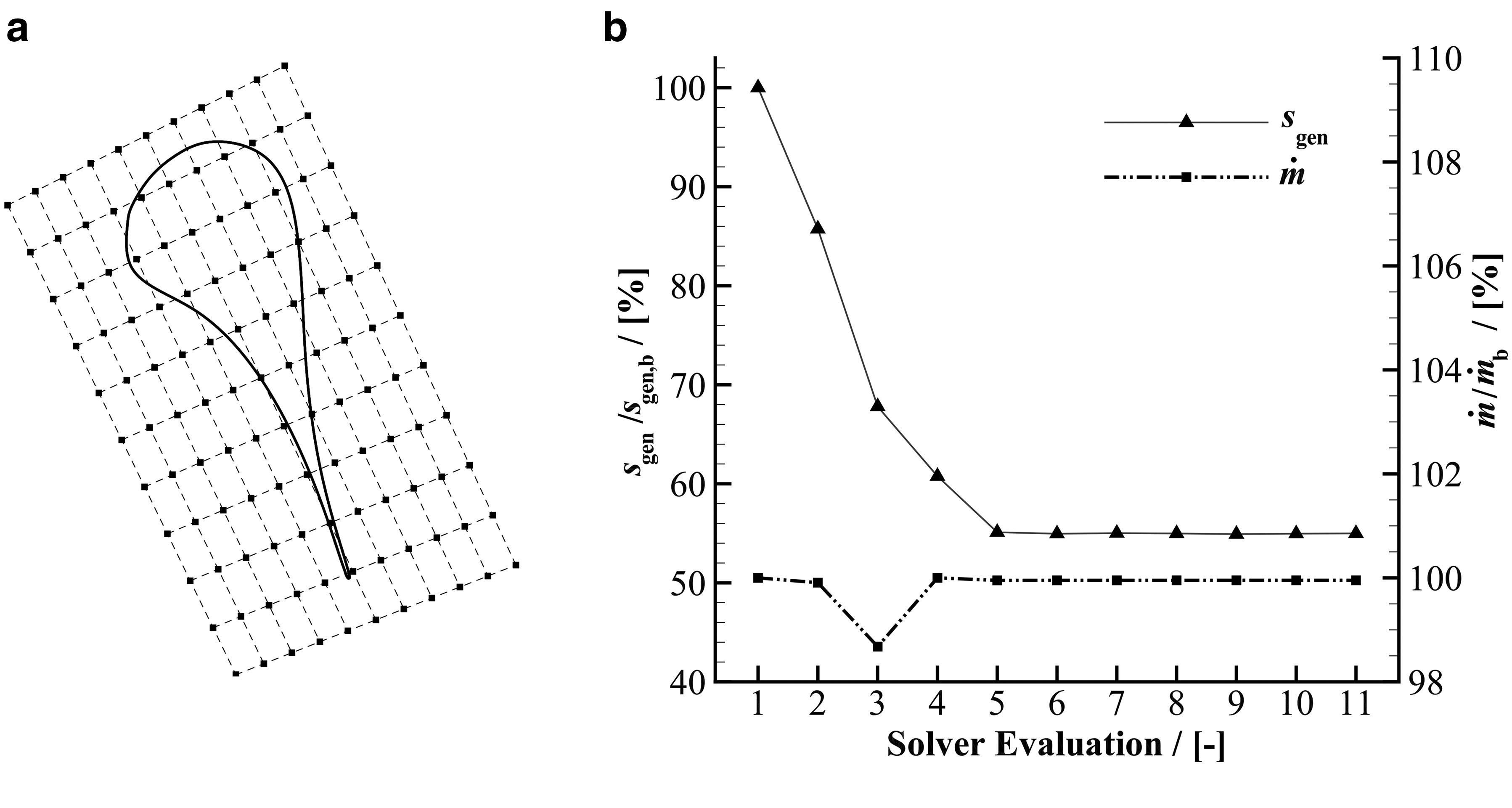
The normalized optimization history in Figure 3 shows that, within 5 iterations, the blade entropy-generation rate is reduced by as much as 45%. A similar reduction is found for the other two performance parameters (44.6% for zp,tot and 47.1 % for zkin), suggesting that the optimal shape is independent from the type of performance parameter selected. The equality constraint on the mass-flow rate is satisfied with an negligible error of 0.01% with respect to the prescribed value.
The Mach contours of both the baseline and the optimal solution are depicted in Figure 4 and Figure 4, and the normalized pressure distributions in Figure 4. In the baseline configuration the simulated flow over-accelerates in the semi-blade region after the outlet divergent section, and this generates an oblique shock on the rear suction side. The over-acceleration is promoted by the continuing increase of flow passage area in the semi-blade region. On the contrary, in the optimized nozzle, the flow acceleration is more pronounced in the divergent channel, after which the flow keeps smoothly expanding through the re-designed straight semi-bladed channel. This results in the complete removal of the shock-wave from the suction-side, and, consequently, in a much more uniform flow at the outlet.
Figure 4.
Flow features of the baseline and the optimized geometry of the supersonic cascade test-case.
a) mach contour of the baseline geometry; b) mach contour of the optimal geometry; c) normalized pressure distribution around the baseline and the optimal geometry.

To gain knowledge of the influence of simulated viscous effects on the design of supersonic ORC cascades, the optimization was repeated using the inviscid adjoint solver. As expected, the use of the inviscid model results into an underestimation of the actual value of the entropy-generation rate, which in the case of the baseline geometry is equal to 129% compared to around 177% predicted by the turbulent solver. Nevertheless, the inviscid and the turbulent optimizations converge to the same optimal geometry, suggesting that the solution of the design problem is driven by the inviscid flow phenomena (i.e., shock-waves). In addition, the computed boundary-layer viscous losses are very similar in the two studied cases. Further numerical experiments demonstrated that this is only valid if the trailing-edge thickness is constrained to its initial value; since, if the thickness is not constrained, the optimization with the turbulent adjoint would lead to a sharp trailing edge, as expected.
Transonic cascade
The second exemplary test case is representative of the fluid dynamic design of transonic cascades commonly found in multi-stage ORC turbines. The operating conditions of the cascade are listed in Table 1. The inlet total pressure and temperature correspond to the inlet turbine conditions of a super-heated MDM thermodynamic cycle; the outlet back pressure was chosen such to obtain a sonic flow at the outlet.
Table 1.
Inlet and outlet boundary conditions values for the transonic cascade test-case.
| Ttot,in | 592.3 | [K] |
| ptot,in | 1.387 | [MPa] |
| βin | 0.0 | [°] |
| pout | 0.90 | [MPa] |
| Itur,in | 0.03 | [-] |
| 100.0 | [-] |
Under the above conditions, the simulated suction-side flow reaches a maximum Mach number of 1.12 at about 90% of the axial-chord length. Afterwards, a shock-wave is generated allowing for a pressure matching downstream of the trailing-edge. The shock causes a sudden increase of the boundary-layer thickness, which eventually results in a more pronounced wake, and, correspondingly, to significant profile losses. Hence, to improve the performance, the cascade was optimized by minimizing its total-pressure loss coefficient. Nevertheless, since the profile-losses are proportional to the flow deflection 13, an unconstrained optimization would ideally converge to a zero-deflection blade. To overcome this issue, the optimization problem was constrained by imposing a minimum tolerable value of the outlet flow angle (βout > 74.0°).
The optimization was performed with a FFD box of degree four in both directions (Figure 5). However, only 20 of the 25 FFD CPs were chosen as a design variables, and the remaining five, belonging to the short-side of the box next to the trailing-edge were kept fixed to prevent unfeasible designs. The flow and adjoint simulations were marched in time for 2,000 iterations on a grid of 17,500 elements using an implicit Euler scheme with a CFL equal to 30.
Figure 5.
Objective function and constraint gradient validation, and optimization history for the transonic cascade test-case.
a) 2D FFD box of degree four on both directions (25 CPs) used for the validation and the optimization; b) comparison between the FD and adjoint gradient values; c) optimization convergence history.
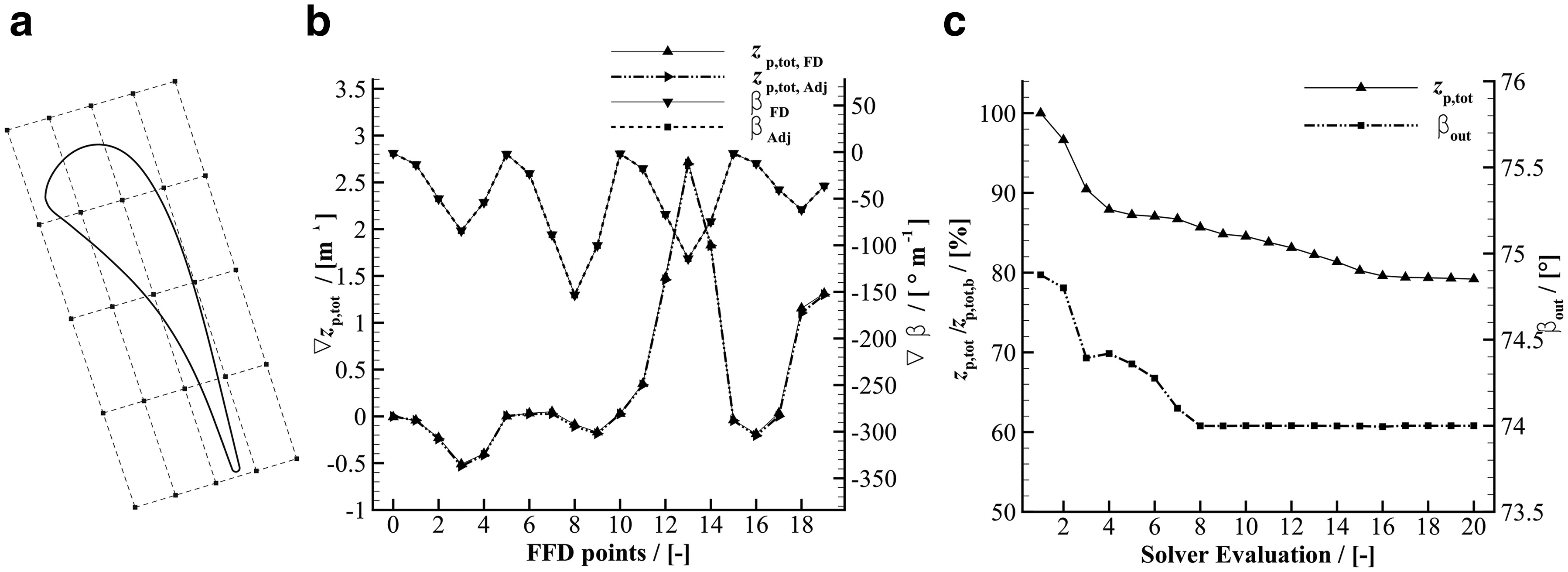
In order to verify the accuracy of the adjoint for predominantly viscous flows, the gradient values was validated against the FD ones using a step-size of 5.0E-06. Figure 5 shows that the norm of the two gradients correlates well, confirming the correct linearization of the RANS flow solver.
As Figure 5 shows, the optimization process converges in 16 iterations. The total-pressure loss coefficient is reduced of about 20% with respect to the initial value, and, as expected, similar reductions are also obtained for the other performance parameters. Furthermore, the optimized flow angle is set to the lower bound of 74° so that, given the constant inflow angle, the flow deflection is reduced to its minimum allowable value.
The baseline and the optimal geometry are compared in terms of normalized pressure distribution in Figure 6. It can be observed that the suction-side velocity peak occurs much more upstream in the optimized blade than in the baseline blade, leading to a smoother flow deceleration on the rear suction side, thus weakening the strength of the shock-wave. This is more evident if the Mach number contours depicted in Figure 6 and Figure 6 are considered. The optimal blade features a reduced outgoing boundary-layer thickness and wake with respect to the baseline. On the contrary, the simulated flow around both geometries display similar characteristics on the pressure side, confirming that most of the losses in transonic ORC cascades are caused by adverse pressure gradients on the rear suction side.
Figure 6.
Flow features of the baseline and the optimized geometry of the transonic cascade test-case.
a) normalized pressure distribution around the baseline and the optimal geometry; b) mach contour of the baseline geometry; c) mach contour of the optimal geometry.

The optimization of the transonic cascade was repeated by using the inviscid flow solver in order to gain insight whether the use of a simpler model can still be advantageous for the design of transonic ORC blades. Interestingly, though the optimization process leads to a reduction of the (inviscid) total-pressure loss coefficient of about 13%, the optimal geometry is practically coincident with the baseline, and the performance improvement predicted by the turbulent solver is negligible (around 1% w.r.t. the initial turbulent value). Apparently, since the main cause of irreversibility are the viscous losses in the boundary-layer, the inviscid adjoint is inadequate for such cases and only a fully viscous adjoint method is suitable for the optimization of transonic ORC cascades.
Influence of the thermodynamic model on the optimal solution
The nozzle of ORC turbines commonly operate with the fluid in thermodynamic states far from ideal gas conditions. As demonstrated in 10, the use of over-simplified thermodynamic models may lead to inaccurate predictions of the main flow features. Table 2 shows, for example, that there are some discrepancies between supersonic cascade performance values calculated with the Ideal Gas (IG) EoS and those calculated with the more accurate PR EoS. Correspondingly, neglecting non-ideal effects in the gradient calculation may lead to sub-optimal blade shape configurations. Nevertheless, as the majority of the available turbomachinery adjoint solvers only implement the polytropic ideal gas model, it is of practical interest to evaluate when the adoption of such model may lead to satisfactory results.
Table 2.
Summarized results of the supersonic-nozzle test-case for different EoSs.
IG | PR | ||
|---|---|---|---|
| zp,tot | 18.36 | 22.78 | [%] |
| 6.384 | 5.953 | [-] | |
| Machout | 1.965 | 1.913 | [-] |
| βout | 77.27 | 76.05 | [] |
To this purpose, the blade geometries documented in the previous section were re-optimized using the polytropic ideal gas model, and the new optimal solutions were compared with the previous ones. The optimal solution calculated using the polytropic ideal gas model is labeled “Optimal-IG,” while that calculated with the PR model maintains the label “Optimal.”
In order to correctly evaluate the performance of the optimized geometry obtained with the flow and adjoint solver linked to the polytropic ideal gas model, the flow solution around such geometry was computed also with the PR model. This solution was then compared with the one illustrated in the previous section. Except the thermodynamic model, all the other test-case parameters (optimization problems, boundary conditions, meshes, FFD box, etc.) were kept the same.
For the supersonic nozzle test-case, an optimal solution is found within 9 iterations. The predicted entropy generation reduction is around 37%, and the constant mass-flow rate constraint is tightly satisfied. As shown in Figure 7, the optimizer is able to calculate a solution for which no shock wave occurs at the rear suction-side of the blade, even if the ideal gas model is used for the computation of fluid properties. The obtained geometry is very similar to the one obtained using the PR model, except for a slight offset, see Figure 7. Even if the geometries are very similar, the calculated performance is different. The performance improvement calculated for the Optimal-IG geometry is 5% lower if compared to that calculated for the Optimal geometry.
Figure 7.
Optimization of the supersonic nozzle geometry using the IG EoS.
a) mach contour of the Optimal-IG geometry; b) comparison between the Optimal and the Optimal-IG geometry; c) compressibility factor for the baseline geometry.
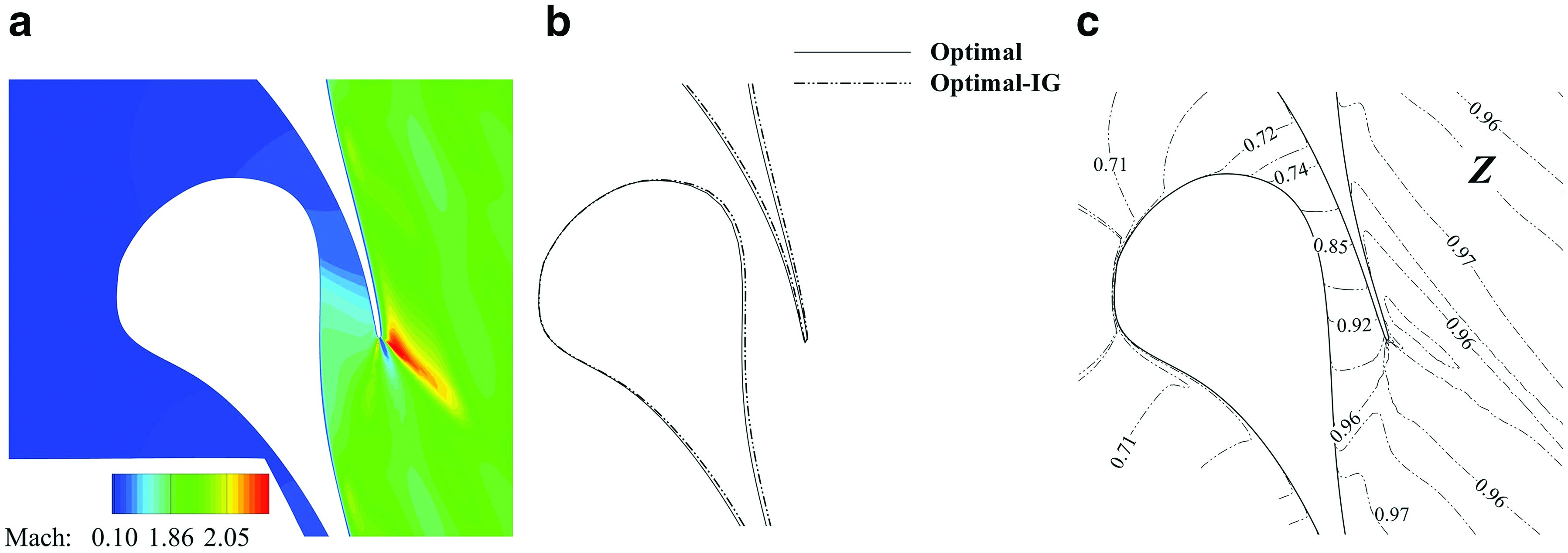
Nonetheless, even the use of the inaccurate ideal gas model allows to calculate a substantial improvement with respect to the baseline, though suboptimal. This result can be explained by observing that the geometry optimization occurs mainly after the throat of the nozzle where the computed compressibility factor is close to unity, see Figure 7.
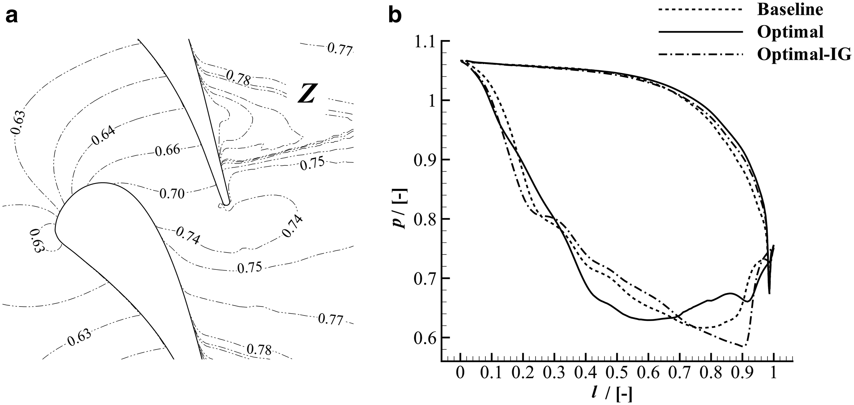
On the contrary, if the cascade is transonic and operates with the fluid completely in the non-ideal thermodynamic regime, the use of the more accurate thermodynamic model is mandatory (Figure 8). The simulation corresponding to the Optimal-IG geometry leads to an estimation of the total-pressure loss coefficient that is higher than that of the baseline (6.49% against 5.27%). As shown in Figure 8, this is due to the fact that the peak velocity is higher, and the normal shock wave on the suction side is stronger.
Conclusion
The technical and economic viability of energy conversion technologies, such as organic Rankine or supercritical CO2 cycle power systems, often depend on the performance of their turbomachinery components, operating partly in the so-called non-ideal compressible fluid dynamic regime. Due to the limited design experience and to the scarce experimental information on NICFD flows, the design of these components greatly benefits from automated fluid dynamic shape optimization techniques. Since the achievement of satisfactory performance of the turbomachinery dictates the use of a large number of design variables, adjoint-based FSO is the only viable technique.
A fully-turbulent adjoint method for the design of nozzles and of turbomachinery operating in the NICFD regime was, therefore, devised. The implementation of the adjoint solver and its application to the design of two exemplary test-cases were presented. The following conclusions can be drawn.
1. Despite the high level of additional complexity due to the need of treating accurate fluid thermodynamic models, it was possible to obtain an exact fully-turbulent adjoint. The linearization of the flow solver was performed with an opensource operator-overloading AD tool (CoDiPack). Given its small overhead in terms of run-time, the AD was applied to the entire flow solver iteration in a black-box manner, thus avoiding a posteriori and ad hoc intervention, which is error-prone.
2. The capability of the new tool was demonstrated by redesigning two typical 2D ORC turbine cascades, in which fluid properties are calculated with the polytropic PR model. In both cases, the optimization performed with the RANS flow and adjoint solver substantially improved the simulated cascades performance, while satisfying the imposed constraints. The optimization process was also repeated assuming inviscid flows. The results emphasize the importance of incorporating the viscous and turbulent gradient contributions, especially for the design of transonic ORC cascades.
3. The potential of the non-ideal compressible RANS adjoint was also shown by comparison with a more conventional ideal gas adjoint method, using the same test cases. The results demonstrate that the simplified approach provides physically inaccurate gradient information leading to sub-optimal cascade configurations, if NICFD effects are moderate. Instead, in case of strong NICFD effects, the calculated performance can be even worse than that of the starting geometry.
Future work will be devoted to the extension of the proposed approach to deal with fluid thermodynamic libraries that are external with respect to the flow solver. In this way, the method can leverage the large number of available software. In addition, the capability of optimizing 3D and multi-stage geometries is being implemented.
Supporting information
Thermodynamic derivatives for the NRBCs
The enthalpy derivatives are computed as
of which the partial pressure derivatives are also used to calculate the speed of sound
The entropy derivatives can be written in terms of the partial derivatives of pressure with respect to temperature and density
The explicit expression of the above partial derivative for different EoS can be found in 51.
Nomenclature
Symbols
U
Conservative or State Variables Vector
F
Flux Vector
Ω
Volume
t
Time
p
Pressure
T
Temperature
µ
Dynamic Viscosity
k
Thermal Conductivity
R
Residuals Vector
c
Characteristic Variables Vector
v
Velocity
ρ
Density
a
Speed of Sound
h
Enthalpy
s
Entropy
β
Flow Angle
u
Internal Energy
z
Loss coefficient
D
Design Variables Vector
J
Objective Function
X
Surface and Volume Mesh Nodes
G
Flow Solver Iteration
M
Surface and Mesh Deformation Matrix
L
Lagrangian
N
Shifted Lagrangian
Flow Adjoint Variables Vector
Mesh Adjoint Variables Vector
R*
Specific Gas Constant
Specific Heat Capacity Ratio
Acentric Factor
Mass Flow Rate
Turbulent Intensity